This is a course review of MATH2000 - Multivariable Calculus and Fundamentals of Analysis taken at CarletonU in the fall of 2022 and winter 2023. The lectures were synchronous but with recorded lectures to accommodate those with COVID-19 or any other illness. This is a review of the first half of the course (the course is 8 months long, 1.0 credit). This blog post is a long one so feel free to skip and read only the course review.
TLDR:
- “introductory” to analysis is interesting but weird to get used to
- Similar to 1052 except extended and more generalized to “higher” dimensions
- Similar to 1052, covers limits, continuity, derivatives, and sequences with a small section on Taylor Polynomials from 2052
- learn how to parameterize curves and surfaces
The review is split into 2 main parts:
- Long Course Description: In-depth talk about the course topic from how I understood it
- Course Review: Solely focuses on the teaching style, difficulty, and anything that would be of interest
Professor: Charles Starling
Course Delivery: Synchronous recorded lectures with synchronous tutorials
Class Size:
- 63 students (Dec 31 2022)
- 53 students (March 28 2023)
Course Description (from website): Higher dimensional calculus, chain rule, gradient, line and multiple integrals with applications. Use of implicit and inverse function theorems. Real number axioms, limits, continuous functions, differentiability, infinite series, uniform convergence, the Riemann integral.
CLICK HERE TO SEE JUST THE COURSE REVIEW
Course Description (LONG) with Commentary:
The course is a two semester long (1.0 credit) course. Similarly to how 1052 focuses on basic analysis and differentiation and 2052 focuses on integration, the same idea applies in MATH2000. The fall semester will focus on basic analysis and differentiation but is no longer constrained to one dimension but to higher dimensions. Hence why this course is called Multivariable Calculus. The 2nd semester (the winter) will focus on integration on higher dimensions.
CLICK HERE TO SEE THE COURSE DESCRIPTION OF THE WINTER SEMESTER
Fall Semester (Open Balls and Differentiability)
Similarly to first year calculus (MATH1052, MATH2052), the lectures go over a lot of proofs. Unlike MATH2100, another course students are required to take and usually taken concurrently, a good understanding of the proofs is not required. As long as you have a rough idea of how the proofs work is sufficient to do well in the course. MATH2000 is interesting in the sense that it extends what you know from first year calculus but “extended” to higher “dimensions”. Starling does a good job to drill into our heads that we are no longer working in one dimension but in higher dimensions. Even the name of the course suggests this (i.e. Multi-variable calculus).
First Year: $f: \mathbb{R}\to\mathbb{R}$
Second Year: $f: \mathbb{R^n}\to\mathbb{R^m}$
As a soft introduction to working with functions of multiple variables, the course first began with talking about some properties of vectors. This topic should be familiar from Linear Algebra. A vector is a set of $n$ numbers belonging to $\mathbb{R^n}$ which is a set of n tuples of real numbers.
$1\in\mathbb{R}$
$(1)\in\mathbb{R^1}$ (usually abbreviated as $(1)\in\mathbb{R}$
$(1, 2)\in\mathbb{R^2}$
Everything about vectors should be review such as vector space properties, doc products and the norm of a vector. What is interesting but obvious is that the norm of a one-dimensional vector is the same as absolute value but in n-dimensional vector space, it is the euclidean distance.
$n = 1: |\vec{x}|= \sqrt{x^2} = |x|$ (absolute value)
$n = 2: |\vec{x}|= |(x_1, x_2)| = \sqrt{x_1^2 + x_2^2}$
What is not a review is the Cauchy-Schwartz Inequality which is a neat inequality that can be used to explain why two vectors are orthogonal if their dot product is 0. The Cauchy-Schwartz Inequality is $|\vec{x}\cdot\vec{y}| \le |\vec{x}|\cdot |\vec{y}|$. The proof for the Cauchy-Schwartz Inequality is not obvious at all and requires some “magical” function to proceed so I would not worry about understanding the proof for Cauchy-Schwartz Inequality at all. What is also interesting about the Cauchy-Schwartz Inequality is that it presents another way to prove the triangle inequality that I suggest trying to understand because it can be helpful for assignments. For instance, $|\vec{x}+\vec{y}|^2 = \sqrt{(\vec{x}+\vec{y})\cdot(\vec{x}+\vec{y})}^2 = (\vec{x}+\vec{y})\cdot(\vec{x}+\vec{y})$ is an expansion you should know for the assignments. One thing to note about the Cauchy-Schwartz Inequality is to be able to differentiate what $|\square|$ means. As stated earlier, it could mean absolute value or it could mean the norm. It depends on what $\square$ is. In the Cauchy-Schwartz Inequality, $|\vec{x}\cdot\vec{y}|$ refers to the absolute value because the dot product operator $\cdot: \mathbb{R}^n \times \mathbb{R}^n \to \mathbb{R}$ outputs a real number. While the other side of the inequality refers to the dot product between the two norms: $|\vec{x}|\cdot |\vec{y}|$. It may be obvious through context but it was something I thought would be important to highlight.
The reason why a Calculus course begins with talking about vectors is that we are dealing with functions of many variables. The input to our functions are no longer a single real number but a tuple of n real numbers. Even the output of the functions we’ll be dealing with in the course may not even be a single real number but a vector such as parameteric curves or some transformation.
The course then resembles a traditional calculus course where the definition of continuity is extended for a function $\vec{f}: \mathbb{R^n}\to\mathbb{R^m}$. Depending on your mathematical background, you might have learned a function is continuous at a point a if the limit from the left and the right are equal and the function is defined at the point a. Students with a stronger mathematical background or stronger mathematical interest would know that continuity can be defined using the delta-epsilon proofs that may have been exposed to in normal calculus but definitely to Math students in the honors/pure program. Luckily for us, the definition of continuty looks identical from first year with the exception of the domain and co-domain of the function.
First Year: a function $f:\mathbb{R}\to\mathbb{R}$ is continuous at $a\in\mathbb{R}$ if $\forall \epsilon > 0$ $\exists \delta > 0 $ such that $\forall x\in\mathbb{R}, |a - x| < \delta \implies |f(a)-f(x)|<\epsilon$
Second Year: a function $\vec{f}:\mathbb{R^n}\to\mathbb{R^m}$ is continuous at $\vec{a}\in\mathbb{R^n}$ if $\forall \epsilon > 0$ $\exists \delta > 0 $ such that $\forall \vec{x}\in\mathbb{R^n}, |\vec{a} - \vec{x}| < \delta \implies |\vec{f}(\vec{a})-\vec{f}(\vec{x})|<\epsilon$
The course then begins to talk about open balls which is a neat concept I was introduced many years ago. As the name implies, it has something to do with open sets and a “ball” (which differs depending what n-dimension you are working with).
Open Ball Centered at $\vec{x}$: for $r>0$ and $\vec{x}\in\mathbb{R^m}$, define the open ball $B_r(\vec{x})=\{\vec{y}\in\mathbb{R}^m: |\vec{x}-\vec{y}| < r\}$
The concept was first introduced to me in a course named Complex Variables (for non-pure math students that I never finished … I was kicked out of the course years ago for not having the prerequisite knowledge). The concept of closed and open sets is very important in the course as we spend a lot of time (about a third of the course) on this topic. For starters, let’s begin talking about what is a ball. A ball is some circular object in the vector space that contains a set of points. An open ball is the set of all points within the radius of the ball. This topic is where some students start to get lost. The concept of open balls is used to talk about a set such as the domain or co-domain in the course or to define what it means for a set to be open, closed, or to define if a point is an interior point or a boundary point.
When talking about domain and co-domain in first-year, we talk about sets and introduce to some basic set notations. It turns out that an open ball in one dimension is simply an interval:
Open Ball Centered at $\vec{x}$ in one dimension: for $r>0$ and $x\in\mathbb{R}$, define the open ball $B_r(x)=\{y\in\mathbb{R}: |x-y| < r\} = (x-r, x+r)$
The reason why it’s called an open ball is because the ball (set) does not contain points that are exactly r units away from the center of the ball. In case you didn’t know, objects like a circle, sphere, or a ball have a boundary of radius r away from the center of the object. Meaning every point in the object is equidistant from the center and therefore any points in the boundary (outline) of the object are r units away from the center. One may say this is an obvious fact but to me personally, the fact that every boundary point on a circle or a sphere is equally far apart from the center as any other boundary point shocked me in university many years ago. This fact never registered in my brain despite being obvious. The term equidistant might ring a bell. Anyhow, I digress (which is a reoccurring theme of my blogs).
What makes open balls fascinating? There are a number of reasons but one of them is that we can rewrite the definition of continuity with open balls. For instance, here’s the definition of continuity of a parametric curve $\vec{f}: I\to \mathbb{R}^n$ where $I\in\mathbb{R}$ is some interval (the domain of the function).
A function $\vec{f}:I\to \mathbb{R}^n$ is continuous at $t\in\mathbb{R}$ if and only if $\forall \epsilon > 0$ $\exists \delta > 0$ such that $\forall s\in B_\delta (t)\cap I \implies \vec{f}(s)\in B_\epsilon (\vec{f}(t))$
Open balls could be used to define many familiar concepts from 1052 such as bounded:
First Year: a set S is bounded if $\exists M > 0$ such that $|x| < M \forall \vec{x}\in S$
Second Year: $S \subseteq B_M(\vec{0})$ (i.e. there exists an open-ball of size M centered at 0 that contains S)
In between talking about open balls and set theory, the topic of parameterization is introduced such as the straight lines, circles, ellipses, and spirals. This topic was something that on the midterm that I thought would not be on it … rip my grades … Anyhow …
The part that is confusing to students is not the definition of an open ball but when we use the definition of an open ball to describe if a point is an interior, closed, or a boundary point or to describe a neighborhood, closure or the set of boundary points.
A point $\vec{x}$ in S is an interior point if $\exists r > 0$ such that $B_r(\vec{x})\subseteq S$
Let’s dissect what cryptic definition. An interior point is a point inside a set that does not lie on the boundary. However, this is not a rigorous definition since we have not defined what it mean to lie in the boundary. While I do not know if this topic lies in analysis or in topology, this course gets much more in-depth describing the properties of sets. The cryptic definition is essentially stating that if $\vec{x}$ is an interior point, we can draw an extremely small open ball such that every point in the open ball lies inside the set S still as seen in the diagram below:
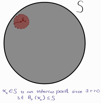
In the diagram, $\vec{x_o}$ is an interior point since there exists an open ball $B_r(\vec{x_o})$, indicated in red, that is contained in the set S, marked in grey. The definition of an interior point can be utilized to describe what it means for a set to be open. One naturally thinks a set is open if there is no strictly defined endpoints in a set. For instance, [0, 1] is closed because there minimum and maxiumum in the interval/set is 0 and 1 respectively. But the set (0,1) is open because the minimum and maximum is not in the set/interval (0,1). The definition of an open set used in the course is the following:
$S \subseteq S^\circ$ is open $\iff \forall \vec{x}\in S$ $\exists r > 0$ such that $B_r(\vec{x})\subseteq S$
For context, $S^\circ$ means the set of all points in S that are interior points of S. So what points are discluded from $S^\circ$? It turns out any points that lie on the edge of the set (i.e. boundary points) do not belong to the set of interior points $S^\circ$. This brings us to the definition of boundary points:
$\forall r > 0, B_r(\vec{x})\cap S\ne \emptyset \land B_r(\vec{x})\cap S^c \ne \emptyset$
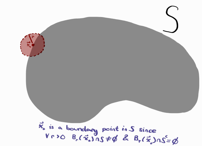
In simpler terms, if a ball centered at some point can contain points both within the set S and its complement (i.e. outside the set), then the point is a boundary point. This definition intuitively makes sense with an illustration. The fact that a ball can be drawn around the boundary points containing points inside and outside the set is what differentiates it from interior points. Let’s relate this new definition of open set with what we know about sets from Highschool. [0, 1] is a closed set where 0 and 1 are boundary points of the set.
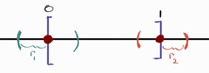
An illustration of the set [0,1] with a ball around the boundary points
The set [0, 1] is closed because we can draw a “ball” (an interval since this is in one dimension) around the point 0 and the point 1 such that the interval will contain points greater than 0/1 and smaller than 0/1 respectively regardless how small the interval $r_1, r_2$ are. It’s interesting to see a formal way to define whether or not a set is closed or open. We’ll explore this again shortly.
The next set of topics is related to limits. The definition for limit hasn’t changed too much from first year but the key difference is that the limit from all directions needs to converge to the same point. The simplest definition for a limit to exist at the point a are the following:
First Year: $\lim\limits_{x\to a} f(x) = L \iff \lim\limits_{x\to a^-} f(x) = \lim\limits_{x\to a^+} f(x) = L$
Second Year: $\lim\limits_{x\to \vec{a}} \vec{f}(\vec{x}) = \vec{L} \iff \lim\limits_{\vec{x}\to \vec{a}} f_i(\vec{x})=L_i \quad \forall 1 \le i \le m$
The following definitions can also be expressed as the following:
First Year: $\lim\limits_{x\to a} f(x) = L \iff \lim\limits_{x\to a} |f(x)-L| = 0$
Second Year: $\lim\limits_{x\to \vec{a}} \vec{f}(\vec{x}) = \vec{L} \iff \lim\limits_{x\to \vec{a}} |\vec{f}(\vec{x}) - \vec{L}| = 0$
Although the definition seems a bit more rigorous, it still lacks rigor. These definition have no rigor and relies on the fact that the reader understands what a limit (i.e. lim) even means. Therefore, the delta-epsilon notation was introduced in first year:
First Year: $\lim\limits_{x\to a} f(x) = L \iff \forall \ \epsilon > 0, \exists \ \delta > 0 $ such that $0 < |x-a| < \delta \ \& \ x\in dom(f) \implies |f(x)-L| < \epsilon$
Second Year: $\lim\limits_{\vec{x}\to \vec{a}} \vec{f}(\vec{x}) = \vec{L} \iff \forall \ \epsilon > 0, \exists \ \delta > 0 $ such that $0 < |\vec{x}-\vec{a}| < \delta $ & $ \vec{x}\in S \implies |\vec{f}(\vec{x})-\vec{L}| < \epsilon$
Similarly, with the definition of continuity, the definition of a function to converge to a point is extended to apply to higher dimensions. Recall in first year, the limit of a function does not exist when the left side and the right side do not converge to the same value. But what about in higher dimensions? It turns out that it is not sufficient enough for a function to converge simply in one curve. The limit must be the same no matter how you approach the point. This may sound confusing, so here’s a simple illustration:
If $f(x) = \frac{xy}{x^2 + y^2}$, then does it converge as (x, y) approaches to the origin?
Unfortunately, the function does not converge when y = x. Details not provided$
I won’t go into the details, you’ll have to take the course to see some examples of what I mean. The next major topic introduced is the Squeeze Theorem, a very important theorem to prove a limit of a complicated function by bounding it between two different functions that converge to the same limit. One powerful tool to prove if a set is closed or open is to figure out if the inverse image or the preimage is open or closed. For a refresher, here are some definitions:
Image of S: If $S\subseteq \mathbb{R}^n$, the image of S is $\vec{f} (S) = \{ \vec{f}(\vec{x}): \vec{x}\in S \}$
Preimage of S: If $U\subseteq \mathbb{R}^n$, the inverse image (or preimage) of U is $\vec{f}^{-1} (U) = \{ \vec{x}\in\mathbb{R}^n: \vec{f}(\vec{x})\in U \}$
One of the biggest reasons why this concept is important is that if a function is continuous, then the inverse image of an open set is open. The same applies to closed sets. Meaning you could easily determine whether a set is closed or open by determining whether or not the codomain, the input set to the preimage, is closed or open. For instance, the set $B=\{(x, y): x^2 +3xy \ge 0 \}$ is closed because $B = f^{-1}([0, \infty))$ and the set $[0, \infty)$ is closed. Thus B is closed. This theorem is a huge time saver. If you choose not to use the theorem, then you’ll be forced to show whether the set is open or closed using open balls.
Similarly to MATH1052, sequences are discussed in the first half of the course. Since we are working in higher dimensions, we need to define what it means for a sequence to converge. There are a few definitions and theorems discussed on sequence convergence such as the good old cauchy sequence but the interesting definition for me is “converging coordinatewise”. The idea is quite simple in the sense that you pick each coordinate in the sequence and see if the coordinate converges using what we know from first year. For context, if a sequence $\vec{x_k} = (x_{k1}, x_{k2}, …, x_{kn})$ converges, each coordinate $x_{ki}$ converge. So if any of the coordinates diverge, then the entire sequence diverges.
The term compactness is again introduced in the course. In this course, a set is compact if the set is closed and bounded. This leads to the “reintroduction” of Bolzano-Weierstrass Theorem on $\mathbb{R}^n$.
Bolzono-Weierstrass Theorem ($\mathbb{R}^n$): If $S\subseteq \mathbb{R}^n$, then S is compact $\iff$ every sequence in S has a subsequence converging in S.
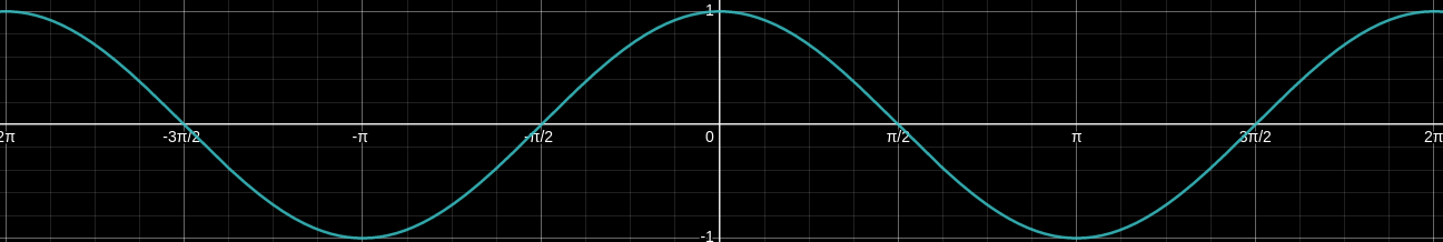
I don’t have much to comment on this theorem but I thought it would be nice to state the theorem since it’s yet another theorem seen in first year in one-dimensional case. The term compactness is important and is going to be seen throughout the course. For instance, the extreme value theorem relies on the set being compact. One confusing aspect of compact is how the image of a continuous function on a compact set is compact. However, the preimage on a compact set is not compact. This can be confusing because the preimage on a open set is open and the preimage of a closed set is closed. But this rule does not apply with compact sets. A simple example is to view a sinusodial function.
A few other important terms in the courses are path, path-connected, and convex. As the name imples, a path is just some continuous curve that connects between two points. Meanwhile, path-connected means you can draw a path between two points that stays in the set. The details is slightly more complicated that I still have a hard time coming up with the proofs:
Path: a path from $\vec{x}$ to $\vec{y}$ in $\mathbb{R}^n$ is continuous function $\varphi : [a,b] \to \mathbb{R}^n$ such that $\varphi (a) = \vec{x}, \varphi (b)= \vec{y}$
Path-Connected: $\forall \vec{x}, \vec{y} \in S, \exists $ a path $\varphi$ from $\vec{x}$ to $\vec{y}$ such that $\varphi$ stays in S
Convex is a more strict version of path connected in that instead of there being any path/curve between two points that stays in S, a convex set requires that any two points in the set can be connected through a straight line that stays in the set. Please recall the parameterization of a straight line because this is extremely important in the course not only to show if a set is convex but for many other concepts in the course such as when solving some problems involving line integrals that will show up in the 2nd half of the course (i.e. winter semester).
If you are a Math-Physics student or have taken PHYS1001, you may be familiar with partial derivatives and gradients already. If you were wondering when Math will introduce the concepts, it’s finally shown in MATH2000. Partial derivatives are simply treating other variable constants and differentiate a function normally. For instance,
\[\partial_x(xy) = y \cdot \partial_x(x) = y (1) = 1 \nonumber\]As this is a calculus course for math majors and not for engineers or science students, we’ll be revisiting what it means to take the partial derivative of a function with respect to some variable using good old limits. Doesn’t everything in this course nicely tie in with 1st year? To explain gradient simply, it’s just a list or a tuple where each number tells you how much the function is changing in respect to some variable. For instance, in the two dimensional case, the first number in the tuple indicates the rate of change in the horizontal direction (i.e. partial derivative with respect to x) while the 2nd number in the tuple indicates the change in the vertical direction (i.e. partial derivative in respect to y). In Mathematical notation: $\nabla f = (\partial_x f, \partial_y f)$
One important note about the topic of gradient and differentiability is that if the function f is differentiable at some point then all of the partial derivatives exist. But I do not think the implication works in the reverse direction. Each partial derivative must be a continuous function for the gradient to exist. In addition, if the function is differentiable at some point $\vec{a}$, then the function is continuous at $\vec{a}$ but the reverse implication is not true. This should have been seen in first year though.
Mean Value theorem is “reintroduced” but this time it is the mean value theorem for convex sets. The term convex is going to show up a lot in this course so you better remember this definition. Uniform continuity pops up again to hunt you. So hopefully you can recall how uniformly continuity works when after the lecture. It turns out that if the gradient of a function is bounded, then the function is also uniform continuous. The term bounded should remind you of compact sets. The next theorem discussed is if a function is continuous on a compact set, then the function is uniformly continuous on the set.
A very key definition in this course is the class $C^k$.
Class $C^k$: a function $f: S \to \mathbb{R} (S\subseteq \mathbb{R}^n)$ is said to be class $C^k$ on S if all of its partial derivatives of all orders less than or equal to k exists and are continuous on some open set containing S
This is going to be seen in so many theorems that it is worth remembering what it means for a function to be in $C^k$. The course then has a short aside on Taylor Polynomials but I am not going to talk about it too much. What is more important for me is to talk about critical points. What is differential calculus without talking about critical points? Critical points tell us when the function has a local min or a local max. It was the interesting part of Highschool calculus, to know where a critical point occurs, whether the critical point was a min or a max, is it local or if it was global. There were interesting word problems associated with these types of questions in Highschool. In honors math, we don’t have word problems and not many application questions, so perhaps it’s not all too interesting to us than to science students. Anyhow, I digress.
Below, I am going to introduce the new definitions of critical point, local max and local min. Do not worry if you cannot follow along, you’ll get to learn if you take the course. This is more for myself. Why would any first year or upcoming 2nd year ever read a long course description, unless they were genuinely curious about the course? I would suggest simply reading the course review and not the course description.
let $f: S \to \mathbb{R}^n$ be differentiable with $S\subseteq \mathbb{R}^n$ be open:
a point $\vec{a}$ is called a CRITICAL POINT if $\vec{\nabla} f(\vec{a}) = \vec{0}$
a point $\vec{a}$ is called a LOCAL MAX if $f(\vec{x}) \le f(\vec{a}) \forall \vec{x}$ in some open ball around $\vec{a}$
a point $\vec{a}$ is called a LOCAL MIN if $f(\vec{x}) \ge f(\vec{a}) \forall \vec{x}$ in some open ball around $\vec{a}$
In first year, to find out if a critical point was a min or a max, we used the 2nd derivative test. In this course, we will be doing something similar in spirit but the approach mixes linear algebra to the mix. There is a matrix called the Hessian Matrix and we compute the matrix which is a matrix consisting of entries that involves taking two partial derivatives of the function with respect to different variables (or the same if it’s along the diagonal). Some neat linear algebra concepts are connected in the course such as symmetric matrices, eigenvalues, and spectral theorem. But the only thing you need to know at this point is the dot product, matrix multiplication, and taking the determinants. You could live without knowing the spectral theorem or finding the eigenvectors when I was taking the course unless I recall it incorrectly (your experience could differ). However, if you are in Math honors, you’ll be also taking ODE (MATH2454) and algebra (MATH2100), so you’ll be forced to review how to find the eigenvalues and the eigenbasis whether you like it or not.
Similarly, how the 2nd derivative test in first year is useless if it returns you a 0, if the determinant of the hessian matrix is 0, the 2nd derivative test for higher dimensions cannot be used. Else:
- $det(H_f(\vec{a})) > 0$ and $f_{xx} > 0 \implies \vec{a}$ is a local min (i.e. $H_f(\vec{a})$ is positive definite)
- $det(H_f(\vec{a})) > 0$ and $f_{xx} < 0 \implies \vec{a}$ is a local max (i.e. $H_f(\vec{a})$ is negative definite)
- $det(H_f(\vec{a})) < 0 \implies \vec{a}$ is a saddle point
The rules are easy to remember because they are analogous to 1-dimensional 2nd derivative test. If $f_{xx} > 0$, that is like saying $f’(a) > 0$, which means the curve opens up forming a smiling face or a valley. Then I can draw a point in the middle of the smile or a valley and that becomes a local min. It’s easy to recall them if you draw a generic curve visually. In regards for local max, $f_{xx} < 0$ which is similar to $f’(a) < 0$ meaning the curve opens down forming a hill. So you can go on top of the hill so it’s a local max.
But what the heck is a saddle point? How I like to see it is to imagine a saddle on a horse meaning the point is where the surface of the function has a flat area in one direction and a sharp ridges in both directions so it neither has a max or min (i.e. it’s not an extremum point). Here’s an illustration from Byju:

The next topic is directional derivatives which as the name implies is what the rate of change would be if you were to move a small distance in the direction of a unit vector from the given point. Directional derivative is defined using limits which I won’t write. The chain rule is discussed but I also won’t be discussing that.
The next major topic is lagrange multipliers which are used to find the minimum and maximum. So what is the difference between lagrange multiplier and the 2nd derivative test you may ask? Lagrange multiplier is to be used when you are given some constraints such as the function operating on a set that is restricted to certain values of x and y or at least that’s how I recalled it.
The next topic is finding vector valued derivative. The difference between the differentiation we were working on earlier was the function was operating on some higher dimensional space to the real numbers (i.e. the image is a subset to the real numbers). But what if the image of the function maps from n-dimension space to a m-dimension space? Then we need to introduce how to compute the derivatives which turns out not to be so difficult. It’s just a matrix where the entries take some partial derivative to a component of the function but can simply be reduced to a column matrix where each entry contains taking the gradient of each component function. Though to be honest, I don’t recall the details so please fact check this.
We also learned about the implicit function theorem but I don’t recall if I skipped the class or the class was canceled so we were supposed to watch the lecture videos. All I can say, I still don’t understand the theorem too well. So I won’t be talking about it.
The final concepts I want to talk about from the fall semester are smooth curves and smooth surfaces. The word smooth should be an indicator of what the function that parameterizes the set is geometrically. It’s essentially a curve or a surface that doesn’t have any hard edges, breaks, or corners. Hence, it’s called smooth. However, the formal definition is not so obvious to decipher:
SMOOTH CURVE: a subset $S \subseteq \mathbb{R}^2$ is called smooth curve if:
i. S is path connected
ii. $\forall \vec{a} \in S, \exists$ an open set N around $\vec{a}$ such that $S \cap N$ is the graph of a $C^1$ function
The definition sounds so cryptic and hard to understand. However, to show a set is smooth, it has to satisfy the above two criteria. To show a curve is smooth on my basic loose-handed definition will be extremely hard because how would one show there are no hard edges or breaks? So let’s break down the importance of the two criteria based on my current understanding (I asked a few people on the CarletonU Math Server to help me out because I only know how to show a set is smooth but did not understand the theory behind it). So I give credit to them but if there is anything incorrect on what I am about to say, it’s likely due to my poor understanding of what they said to me:
i. S is path-connected
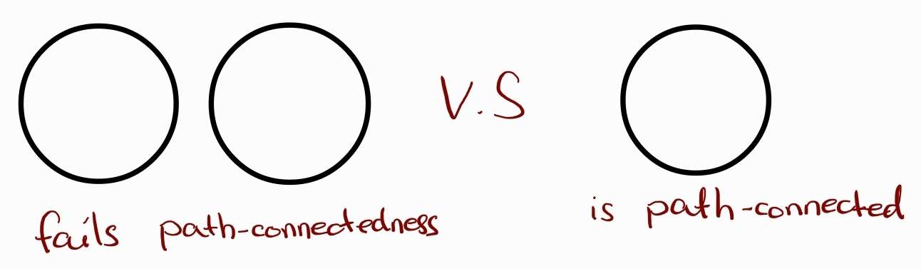
Why is path connected even a condition for a set to be smooth. Initially I thought it was to ensure the function that parameterizes the set would be continuous. Maybe there is some truth behind this but the condition is there to ensure the set is one object and not a union of two disjoint sets like a pair of non-intersecting circles.
ii. $\forall \vec{a} \in S, \exists$ an open set N around $\vec{a}$ such that $S \cap N$ is the graph of a $C^1$ function
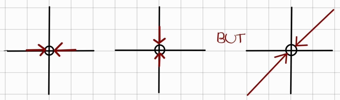
The second criterion in the definition is to ensure there are no sharp edges and that the object will be one dimensional (hence why it’s a curve). An example someone gave me was to graph a literal + (plus) symbol in the graph. So the set would be $S=([-1,1]\times{0})\cup({0}\times [-1,1])$. The center or the origin would fail the 2nd condition because the set around the origin intersected with S are not differentiable. Visually, it’s obvious that the origin is an issue because there are sharp corners. But through this definition, it’s not so obvious aside from the fact that the limits as x approaches the center differ and hence is not differentiable.
Practically speaking, to show a set is smooth:
i. find a parameterization of the set and state that since the parameterization is continuous, the set is path-connected
ii. find the zero set of the set and ensure its gradient is not 0
The definition for a smooth surface is different but I want to move along to describing what was covered in the winter semester.
Winter Semester (Integration in Higher Dimensions and on Vector Fields)
Integration of Functions
The start of the semester parallels with how MATH2052 begins by reviewing Darboux Sums and the definition of integrability. Unfortunately, Folland, the author of the textbook Advanced Calculus, prefers to call Darboux Sums and Darboux Integrals as Riemann Sums and Riemann Integrals even though it’s Darboux. In addition, Folland uses different notation for Lower and Upper Darboux Sums/Integrals. Here are some notation translation if I recall correctly what we used last year:
Upper Darboux Sum: $U(f,p) = S_pf = \sum\limits_{k=1}^n M(f, [t_{k-1}, t_k])(t_k - t_{k-1}) = \sum\limits_{k=1}^n M_k(t_k - t_{k-1})$
Lower Darboux Sum: $L(f,p) = s_pf = \sum\limits_{k=1}^n m(f, [t_{k-1}, t_k])(t_k - t_{k-1}) = \sum\limits_{k=1}^n m_k(t_k - t_{k-1})$
Notice how $U(f,p)$ is now $S_pf$ where the letter S is supposed to represent sum from my understanding. If we are denoting upper sum, it’s a captial S and if we are denoting for a lower sum, it’s a lowercase s. While the notation is clear in the text, the notation is not ideal because it is easy to be confused between the two when the notation is written by hand. Another issue with this new notation is that there is a loss of information with the notation of max M and min m. In case you forgot what the definition of max and min are, here’s the definition from first year.
For a set $S \subseteq [a,b]$ and $f$ is bounded on [a,b]:
Max: $M(f, S) = sup\{f(x): x\in S\}$
Min: $m(f,S) = inf\{f(x): x\in S\}$
These determine the height of your rectangles for each partition. But the new notation used in the course is bad because it’s vague and loose. In first year, the max and min “function” requires two parameters, the function and the subset that the function maps to. However, the new notation omits the first parameter, the function. So how would one know
what function is being applied in the max or min. It is clear from context what function is binded to the min or max since the lower or upper darboux sum does require you to specify the function. In my opinion, it gets a bit wonky when you are trying to show that a function g that is strictly greater than a function f using this new notation because both functions have the same min or max. So you need to introduce a new min or max for one of the functions to avoid confusion.
What about integrability? The idea and every lemma and theorem from first year are the same inclusing the Cauchy Criterion. As mentioned before, the notation for integrability did change. This new notation is actually more intuitive than our first year notation.
Upper Darboux Integral: $U(f) = \bar{I}_a^b = inf\{S_pf: $P is a partition of $[a,b]\}$
Lower Darboux Integral: $L(f) = \underline{I}_a^b = sup\{s_pf: P$ is a partition of $[a,b]\}$
Similar to the new notation for Darboux Sums, the letter is more intuitive as I stands for integrability. I am so glad the author did not use a lowercase i to state Lower Darboux Integral. The bar and underline is also intuitive and also provides us information on where the function f is bounded. However, the function is ommitted … unless I have my notes written incorrectly.
A theorem in class proposes that every continuous function is integrable which sounds reasonable without even looking at the proof. One would think that any continuous curve will have some area that can be measured. What about discontinous functions? From MATH2052, you may have recalled that a function that is discontinuous at a finite number of points is still integrable. However, infinite sets such as a converging sequence can also be integrable as well. This may sound very counter-intuitive and yes we do have to be careful about this claim. There are two criteria that must be satisfied. We have no formal theorem in first-year to cover this case. The theorem goes along like this:
THM 4.13: If f is bounded on [a,b] and the set of points in [a,b] at which f is discontinuous has zero content, then f is integrable on [a, b]
To understand this theorem, we need to first understand what zero content is.
Zero Content: a set $Z\subseteq \mathbb{R}$ has zero content if $\forall \epsilon > 0, \exists$ in tervals $I_1, I_2, …, I_n$ such that:
- $Z \subseteq \bigcup\limits_{i=1}^{n}I_i$
- $\sum\limits_{i=1}^{n}$len($I_i$) < $\epsilon$
Informally,
zero content means small enough to be negligible, for purposes of integration. – UofT MAT237 Notes
Essentially, if a bounded function has zero content, the discontinuity is so small that it is negligible. Hence why we can ignore the discontinuity and still be able to calculate the integral of the function between [a, b]. I for some reason has some fixation trying to visualize what zero content is but as Folland says, the reader should not attach undue importance to it. I spent way too much time trying to conceptualize this definition fruitlessly during the course. So what is the definition of zero content telling us?
a bounded function could still be integrable even if it’s infinitely discountinuous as long as:
- the discontinuity can be covered by finitely many intervals AND
- the total length of the intervals is arbitrarly so small that it’s insignificant
As with any calculus course, the fundamental theorem of calculus is once again mentioned but this time, it’ll also mention about zero content. The course continues to chapter 4.2 of the textbook which is integration on higher dimensions. The darboux sums and darboux integrals are extended to higher dimensions by treating the partitions to be rectangles instead of just intervals in one-dimension.
I’ll be transparent and say that the material I am about to mention from now on is something I am not comfortable with so take what I say with a grain of salt and fact-check whatever I am about to say.
The definition of characteristic function is given which is essentially a piecewise function that returns 1 if the point is in the set and returns 0 otherwise.
Characteristic Function: given $S\subseteq \mathbb{R}^n$, the characteristic function of S is $\chi_s(\vec{x}) = \begin{cases}1&\mbox{ if } x\in S \\\\0&\mbox{ if } x\not\in S\end{cases}$
What is the point of this function you may ask? In higher dimensions, we care about integrating a function whose domain is not a rectangle. We extend the set in which we integrate by bounding it with a sufficiently large rectangle box R containing a non-rectangular set S. However, this will introduce a bigger set to integrate over than desired. Hence why the characteristic function was introduced. The characteristic function allows us to integrate over the rectangle without worry since anything that is not in the set is 0. So we have the integral:
$\int\int_S fdA = \int\int_R f\chi_s dA$
The next topic introduced is Jordan Measurable which I guess was introduced to extend the definition of the integral beyond just rectangles. But it’ll be important for the upcoming theorems in the course.
Jordan Measurable: $S\subseteq \mathbb{R}^2$ is Jordan Measurable if $\partial S$ has zero content
You’ll have to take the course to get a more detail look at why we introduce Jordan Measurabe. As I do not have good understanding of the material, I’m just going to skip a lot of details and start talking about Iterated Integrals.
If you ever asked someone who took any version of multivariable calculus, they are going to tell you that taking the integral of a n-dimensional space is just repeated single variable integration where you treat the other variables as constants like what we do when computing partial derivatives. Fubini’s Theorem is what allows us to do this. In the 2-dimensional case, we can think of it as splitting the region into very thin vertical/horizontal slices and then calculate the area of each vertical/hoirzontal slice. The sum of the area of all the slices will be the area of the region. One nice thing about integration is that you can change the order of integration and you should get the same result if the function is nice like a continuous function.
$\int\limits_0^1\int\limits_{-1}^2\int\limits_0^3 xyz^2dzdydx = \int\limits_{-1}^2\int\limits_{0}^3\int\limits_0^1 xyz^2dxdzdy$
Note that we start by dealing with the innermost integral and proceed to solve the single variable integration outward one by one till we get to the outermost integral (i.e. the last integral remaining in the equation).
$\int_0^2\int_0^1 xy dydx = \int_0^2(\int_0^x xy dy)dx = \int_0^2 x(\frac{y^2}{2}\bigm|_0^x) dx = \frac{1}{2}\int_0^2 x(x^2 - 0^2)dx = \frac{1}{2}\int_0^2 x^3dx = \frac{1}{2}(\frac{x^4}{4}\bigm|_0^2) = \frac{1}{8}(2^4 - 0^4) = 2$
The next type of integration done in the course is what is called Change of Variables. This sort of reminds me of Special Relativity which I dropped in the sense that we can transform or change our frame of reference and the system should remain invariant (i.e. the physical reality does not change even if a transformation is applied onto the system). So if we were to scale, shift (translate), or rotate our coordinate system, the area or volume under the region should be invariant (not changing). It turns out that changing our coordinate system can make our lives easier. The Change of Variables has the form:
$\int_I f(x)dx = \int_{g^{-1}(I)} f(g(u))|g’(u)|du$
When working on integration problems from here on, it’s best to see examples and practice which I did not do enough of … Anyhow, there are three big coordinate systems you need to remember for this course:
- Polar Coordinates
- Cylindrical Coordinates
- Spherical Coordinates
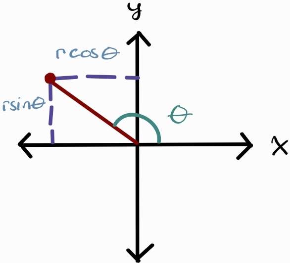
Polar coordinates is something you should be somehwat already familiar with. When working on complex numbers, polar coordinates is in the form $r(\cos\theta + i\sin\theta)$. So we have the following:
- $x = r\cos\theta$
- $y = r\sin\theta$
- $r = \sqrt{x^2 + y^2}$
Here’s where I get confused where the heck the special factor comes from. The change of variables can be rewritten as the following:
$\int_I f(x)dx = \int_{g^{-1}(I)} f(G(u))|det DG(u)|du$
This definition introduces the Jacobian of the change of variables $|det Dg|$. This magically appears out of nowhere, at least to my mind. I do not know as to how the Jacobian of the change of variables appears and this did cause a great confusion in my head. However, you can safetly ignore the derivation and accept the equation as is. Jacobian matrix is something you may or may not have seen in first year linear algebra but it’s somewhat implied you should know this in MATH2454 ODE I believe.
Using this new equation, we can determine how to reorient the problem to use polar coordinates as follows:
$(x,y) = G(r, \theta) = (r\cos\theta, r\sin\theta)$
so
\[\begin{aligned} \rvert det Dg(r, \theta)\lvert &= \Biggm\rvert det\begin{bmatrix} \frac{\partial}{\partial r}x & \frac{\partial}{\partial \theta}x \\ \frac{\partial}{\partial r}y & \frac{\partial}{\partial \theta}y \end{bmatrix}\Biggm\lvert \\ &= \Biggm\rvert det\begin{bmatrix} \frac{\partial}{\partial r}x & \frac{\partial}{\partial \theta}x \\ \frac{\partial}{\partial r}y & \frac{\partial}{\partial \theta}y \end{bmatrix}\Biggm\lvert \\ &= \Biggm\rvert det \begin{bmatrix} \frac{\partial}{\partial r}r\cos\theta & \frac{\partial}{\partial \theta}r\cos\theta \\ \frac{\partial}{\partial r}r\sin\theta & \frac{\partial}{\partial \theta}r\sin\theta \end{bmatrix}\Biggm\lvert \\ &= \Biggm\rvert det \begin{bmatrix} \cos\theta & -r\sin\theta \\ \sin\theta & r\cos\theta \end{bmatrix}\Biggm\lvert \\ &=\rvert\cos\theta(r\cos\theta) - (-r\sin\theta)(\sin\theta)\lvert \\ &=\rvert r\cos^2\theta + r\sin^2\theta \lvert \\ &=\rvert r(\cos^2\theta + \sin^2\theta) \lvert \\ &=\rvert r \lvert\\ &= r \qquad \text{,since $r \ge 0$} \end{aligned}\]Hence, the integral when reoriented in polar coordinates, we have:
Polar Coordinates: $\int\int_S fdA = \int\int_{G^{-1}_\text{polar}(S)} f(r\cos\theta, r\sin\theta)rdrd\theta$
Cylindrical coordinates is similar to polar coordinate but with one major disinction, a cylinder has a height. Meaning there is a 3rd-dimension along the z-axis. So we now have: $(x, y, z) = G(r, \theta, z) = (r\cos\theta, r\sin\theta, z)$. We can now compute the Jacobian for cylindrical coordinates to determine the equation for cylindrical coordinates:
\[\begin{aligned} \rvert det Dg(r, \theta, z)\lvert &= \Biggm\rvert det\begin{bmatrix} \frac{\partial}{\partial r}x & \frac{\partial}{\partial \theta}x & \frac{\partial}{\partial z}x\\ \frac{\partial}{\partial r}y & \frac{\partial}{\partial \theta}y & \frac{\partial}{\partial z}y\\ \frac{\partial}{\partial r}z & \frac{\partial}{\partial \theta}z & \frac{\partial}{\partial z}z\\ \end{bmatrix}\Biggm\lvert \\ &= \Biggm\rvert det\begin{bmatrix} \frac{\partial}{\partial r}r\cos\theta & \frac{\partial}{\partial \theta}r\cos\theta & 0\\ \frac{\partial}{\partial r}r\sin\theta & \frac{\partial}{\partial \theta}r\sin\theta & 0\\ 0 & 0 & 1\\ \end{bmatrix}\Biggm\lvert \\ &= \Biggm\rvert 0 - 0 + 1 \cdot det \begin{bmatrix} \cos\theta & -r\sin\theta\\ \sin\theta & r\cos\theta\\ \end{bmatrix}\Biggm\lvert \\ &= \Biggm\rvert det \begin{bmatrix} \cos\theta & -r\sin\theta\\ \sin\theta & r\cos\theta\\ \end{bmatrix}\Biggm\lvert \qquad\text{(same as polar coordinates)}\\ &= r \end{aligned}\]As expected, adding a height does not affect the scale on the xy-plane. Hence why the Jacobian remains identical to polar coordinates. Hence,
Cylindrical Coordinates: $\int\int_S fdA = \int\int_{G^{-1}_\text{cyl}(S)} f(r\cos\theta, r\sin\theta, z)rdrd\theta dz$
The final coordinate system introduced is the spherical coordinates. This is much trickier to understand so I know some students opted to remmeber the formula. A cylinder is similar to a sphere in the sense that both shapes are circular. But a sphere is equidistant from the center of the sphere. Meaning, all 3 coordinates: x, y, z are transformed. It is no longer sufficient to have a single angle to represent the transformation. If I am not lazy, I’ll program some animations in Python for you to visualize how the spherical coordinates is formed. (If you do not see any animations, it means I was too lazy to write one. It does take a while since I am terrible at using Manim).
In cylindrical coordinates, we had $(r\cos\theta, r\sin\theta, z)$. But the height of a sphere cannot simply be represented by the value of z. When we transform the coordinate system to spherical, we need to consider that the z coordinate is also transformed.
For now, let’s focus on the first two coordinates: x and y coordinates. If you understand polar cylindrical (and therefore polar) coordinates, you can agree that x and y has some relation with $r\cos\theta$ and $r\sin\theta$:
\[x \quad \alpha \quad r\cos\theta \nonumber\\ y \quad \alpha \quad r\sin\theta\]However, this transformation only maps in the xy plane. This makes intuitive sense since this derivation came from polar coordinates which operate on the xy plane (technically, it’s the $Re z = x$ and $Im z = iy$ plane). Therefore $\theta$ is the angle along the xy plane:
However, this does not give us the height of the object in 3-dimensional space. Therefore, we need to introduce a z-coordinate and a new angle to represent this new height (since z coordinate has been transformed in spherical coordinates).
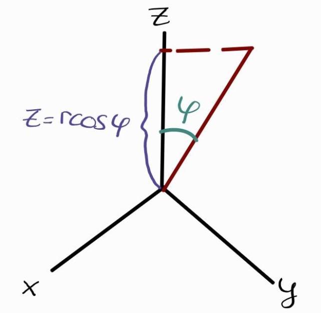
Fig 1: An illustration of the purpose of $\varphi$ in the z-axis
Similarly how the angle $\theta$ starts from the x-axis, $\varphi$ starts from the z-axis. One many notice that to represent any point in the xy plane, $\theta$ needs to be between 0 to 2$\pi$ radians. However, $\varphi$ is restricted from 0 to $\frac{\pi}{2}$ radians (i.e. 0 to $90^\circ$). The purpose of the z-axis is to represent the height. It is unnescessary for $\varphi$ to exceed $90^\circ$ because $\cos\varphi$ is symmetric (i.e. $\cos(\varphi) = \cos(-\varphi)$) as seen below:
Recall from Highschool the SOH CAH TOA rule. To obtain the transformed z-coordinate, we are interested in only the height (the vertical component) which happens to be $r\cos\varphi$. The xy-plane does not affect the height of the point at all. Therefore we have,
\[x \quad \alpha \quad r\cos\theta \nonumber\\ y \quad \alpha \quad r\sin\theta \nonumber\\ z = r\cos\phi\]Notice how the point also has a horizontal component in figure 1 above when I was trying to illustrate the purpose of $\varphi$ on the z-axis. It turns out that when we transformed the coordinates to spherical, $\varphi$ also impacts x and y components. The effect of the z-axis on x and y coordinates is a scalar transformation which can be modelled by the horizontal component $\sin\varphi$ (notice how we ommitted the constant factor r as this was already taken into consideraiton by the transformation to polar coordinates). We now have:
\[x = r\sin\varphi\cos\theta \nonumber\\ y = r\sin\varphi\sin\theta \nonumber\\ z = r\cos\phi \nonumber\\ G = (r, \theta, \phi) = (r\sin\varphi\cos\theta, r\sin\varphi\sin\theta \nonumber, r\cos\phi)\]All that is left is to compute the Jacobian so that we can finally figure out the equation of change of variables for spherical coordinates:
\[\begin{aligned} \rvert det DG(r, \theta, \phi)\lvert &= \Biggm\rvert det\begin{bmatrix} \frac{\partial}{\partial r}x & \frac{\partial}{\partial \theta}x & \frac{\partial}{\partial \varphi}x\\ \frac{\partial}{\partial r}y & \frac{\partial}{\partial \theta}y & \frac{\partial}{\partial \varphi}y\\ \frac{\partial}{\partial r}z & \frac{\partial}{\partial \theta}z & \frac{\partial}{\partial \varphi}z\\ \end{bmatrix}\Biggm\lvert \\ &= \Biggm\rvert det\begin{bmatrix} \frac{\partial}{\partial r}r\sin\varphi\cos\theta & \frac{\partial}{\partial \theta}r\sin\varphi\cos\theta & \frac{\partial}{\partial \varphi}r\sin\varphi\cos\theta\\ \frac{\partial}{\partial r}r\sin\varphi\sin\theta & \frac{\partial}{\partial \theta}r\sin\varphi\sin\theta & \frac{\partial}{\partial \varphi}r\sin\varphi\sin\theta\\ \frac{\partial}{\partial r}r\cos\varphi & \frac{\partial}{\partial \theta}r\cos\varphi & \frac{\partial}{\partial \varphi}r\cos\varphi\\ \end{bmatrix}\Biggm\lvert \\ &= \Biggm\rvert det\begin{bmatrix} \sin\varphi\cos\theta & -r\sin\varphi\sin\theta & r\cos\varphi\cos\theta\\ \sin\varphi\sin\theta & r\sin\varphi\cos\theta & r\cos\varphi\sin\theta\\ \cos\varphi & 0 & -r\sin\varphi\\ \end{bmatrix}\Biggm\lvert \\ &= \Biggm\rvert \cos\varphi det\begin{bmatrix} -r\sin\varphi\sin\theta & r\cos\varphi\cos\theta\\ r\sin\varphi\cos\theta & r\cos\varphi\sin\theta\\ \end{bmatrix} - 0 + (-r\sin\varphi)det \begin{bmatrix} \sin\varphi\cos\theta & -r\sin\varphi\sin\theta \\ \sin\varphi\sin\theta & r\sin\varphi\cos\theta \\ \end{bmatrix}\Biggm\lvert \\ &=\rvert r^2\cos\varphi(\sin\varphi\cos\varphi\sin^2\theta - \sin\varphi\cos\varphi\cos^2\theta) - r\sin\varphi(r\sin^2\varphi\cos^2\theta - (-r\sin^2\varphi\sin^2\theta)\lvert\\ &= \rvert r^2\cos^2\varphi\sin\varphi(\sin^2\theta+\cos^2\theta) - r^2\sin\varphi\sin^2\varphi(\cos^2\theta + \sin^2\theta)\lvert\\ &= \rvert -r^2\sin\varphi(\cos^2\varphi + \sin^2\varphi)\lvert\\ &= \rvert -r^2 \sin\varphi \lvert \\ &= r^2 \sin\varphi \end{aligned}\]Thus,
Spherical Coordinates: $\int\int_S fdA = \int\int_{G^{-1}_\text{sph}(S)} f(r\sin\varphi\cos\theta, r\sin\varphi\sin\theta, r\cos\varphi)r^2\sin\varphi drd\theta dz$
That was a lot of work to derive these three coordinate systems. Hence, most students just simply remember the coordinate system with a rough understanding how one would derive the coordinate system. The next topic revisits improper integrals which I won’t get into because that should be a review from last year. Except in MATH2000, we deal in higher dimensions.
Integration of Vectors
The course now begins on Vector Calculus. We are no longer constrained to finding area under the graph of some function $f: \mathbb{R}^n \to \mathbb{R}$. The course shifts its focus to integration functions $F: U\subseteq\mathbb{R}^n\to\mathbb{R}^n$ which describes a vector field. In other words, a vector field is a function where the domain and range have the same dimensions. This is not a Physics class but you will be seeing a lot of applications and relation to Physics. Personally, I view a field as the forces that determines the path (direction) and magnitude of any object dropped into any area under the field’s influence. We can think of the graviational field or the electric field for instance. Earth’s gravitational field pulls any objects towards it but with different intensity. If I was on the surface of Earth or even on Earth’s low orbit, the gravitational pull exerted by Earth is strong compared to a satellite orbiting around Mars for instance. But visualizing a vector field using Gravity is dull to me. How I like to visualize is a whirlpool where arrows are drawin in spiral paths (sorts of reminds me of phase plane portraits in MATH2454 ODE).

If I was to drop any object down any point in the field, you would be able to predict the trajectory of the object from the vector field. At least that’s how I thought of it but I am not into analysis and I also didn’t exactly do that well in the course. So take my words with a grain of salt.
It is not important at all to know the application of Physics in this course. It’s just neat to see how interdisciplinary Mathematics is. Regardless, I purged all my Physics knowledge right after I made the decision to switch into Math so whatever I am saying could be very wrong. The first major concept in vector calculus that was introduced was arc length which you could be familiar with if you have taken MATH1004, Calculus for Engineers, if for some odd reason your academic background was in Engineering prior to switching (or trying to switch) into Math. Arclength as the name implies allows you to measure the length of a curve such as calculating the circumference of a circle. Calculating arclengths is not difficult at all, just remember the formula and how to parameterize the curve. This topic was interesting because you could apply calculus to determine length of shapes and curves that exist in reality even if there are much more simpler ways to do that.
The next topic is related to arc lengths but for higher dimesnions called line integrals. Before I go into analogies, it might be clear if I showed you the equations for arc lengths and line integrals so you compare between the two:
Archlength: $\int_C fds = \int_a^b |g’(t)|dt$
Line Integral (Scalar): $\int_C fds = \int_a^b f(g(t))|g’(t)|dt$
As one can observe, arclength is a special case of a scalar line integral where the arclength of our curve is $\int_C 1ds$ (i.e. the scalar function being integrated is 1). One way to view line integrals of a scalar function is as follows:
$\int_C f ds = (\text{arclength of C}) \times (\text{average of f over C})$
However, this is a non-rigorous and imprecise definition of what it means to compute the line integral of a function. One way to think of line integral is to think about shovelling snow where the heights differ along the path. The amount of snow you shovel is dependent on where you shovel (i.e. depth differs), how far you shovel and etc. It represents an accumulation (i.e. snow) above the path. This is an anology that Dr. Trefor Bazett, a professor in Canada and a youtuber, introduced to give an intuition what line integrals mean. Starling’s introduction was a bit confusing at first till someone mentioned it seemed like taking the area of a curtain by computing the height of the curtain as you go along the curtain. One interesting thing about line integrals is that the direction (called orientation) in which you traverse the path does not matter which makes intuitive sense. But what if instead of working with scalar functions, we work on vector functions? Would the direction matter?
As most will say, computing the line integral of a vector field is much more interesting than a scalar function due to its many application in physics. Recall a vector field allows us to know both the direction and magnitude of a particle at any point in the field. Such vectors can be thought of as force or velocity as both properties have a direction and magnitude which we can use to compute the work done as the particle traverses through a path. If you have taken PHYS1001, you will know that work can be defined more than just the product of force and distance:
\[W = Fd = \int_C \vec{F} \cdot d\vec{x} = \int_C (F_1dx_1 + ... + F_n dx_n) = \int_a^b F(g(t))\cdot g'(t)dt \nonumber\]Unlike line integrals of scalar functions, the orientation (direction) does matter. However the difference between the orientation happens to be the negation of the other. Line integrals could be tricky to compute which is where the next concept, Green’s Theorem, comes into play. I didn’t realize the relation between line integrals and Green’s Theorem until recently. Green’s Theorem can be used as a tool to convert a line integral around a simple closed curve into a double integral over a region enclosed by that curve. Solving a single integral may sound easier than a double integral but that is not always the case. Before I go into anymore details, I probably should introduce what Green Theorem even is:
Green’s Theorem: Let $S \subseteq \mathbb{R}^2$ be a regular region with piecewise C’ boundary S. If $\vec{F=(P,Q)}$ is a C’ vector field on S then: $\oint_{\partial S} \vec{F}\cdot d\vec{x} = \int\int_S (\frac{\partial Q}{\partial x} - \frac{\partial P}{\partial y}) dA$
All of this Math jargon might be confusing but here’s the closest meme I could fine that Starling showed us to understand Green’s Theorem (practically the same meme but it was how engineers saw Green’s Theorem instead of Physicists)

I will attempt to explain Green’s Theorem in more detail and in another approach soon but let’s take a few steps back. One way to view line integrals over vector fields is to think of the force flowing. For instance, think of water flowing across a smooth surface. A line integral can compute the flow of water moving along (or tangential to) the curve. If the curve is closed (i.e. path connected and starts & closes at the same point like a loop), then the flow circulates. What Green’s Theorem is telling us that we can calculate the total flow of the vector field across the closed curve by seeing what happens inside the loop.
I have skipped a lot of details and you may be confused as to why I started to talk about flow. Hopefully in due time, it’ll make sense but I also have poor understanding of material as stated earlier. So hopefully, I haven’t said anything too outrageous yet. You may have noticed that I skipped a lot of details in between such as what it means for a path to be independent, what a regular region is or what does it mean for a vector to be conservative. So I’ll explain what those are (for myself):
A vector $\vec{F}$ is conservative if $\vec{F}=\vec{\nabla}f$ for some f
F is conservative $\implies \int_{C_1}\vec{F}\cdot d\vec{x} = \int_{C_2} \vec{F}\cdot d\vec{x}$ where $C_1$ and $C_2$ are two path that start and end at the same points
Do not fret if the definition of conservative is scary. The definition of conservative from Physics remains the same in Math. As a review, a force is conservative if the work done by the force on a particle is independent of the particle’s path. Essentially, all that matter is where the particle that the force is acting on starts and ends (i.e. the end points of our integral). Some examples of conservative fields are gravitational and electrical field. $\vec{F}=\vec{\nabla}f$ is a key property for a vector to be conservative and can be used as a quick test to see if the vector is conservative or not. What we are saying is that if a vector can be expressed by some scalar potential function, it is conservative.
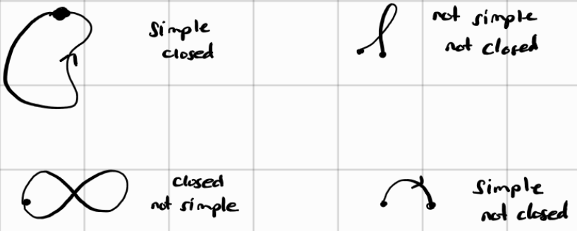
Before I can explain what the word regular region that appears in the definition for Green’s Theorem is, we first need to know what it means for a path to be SIMPLE.
SIMPLE: a path C is SIMPLE if it has no self-crossings (except possibly at the start and end)
This is best illustrated with a diagram:
Now that we know what a simple path is, we can now explain what a regular region is:
Regular Region: a regular region $S\subseteq \mathbb{R}^n$ is called a REGULAR REGION if it is compact and $S=(\overline{S^\circ})$
As always, examples and illustrations explain a thousand words:
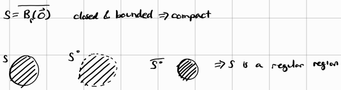
What is interesting about regular regions is the implication that no information is lost when you take the interior of a region. In other words, all the information you need to recover the closed region is contained in the interior region itself. This has significance I would imagine in information theory in the sense that you can store less information and still recover the original information which we call lossless compression. Though I am no expert in information theory. If this talk about losless compression makes no sense, perhaps it will (hopefully) if you look at the next example:
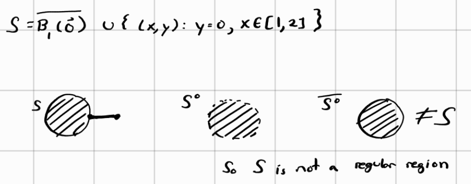
The example above is an example of what a non-regular region is. As you can see, the original region contains a line segment sticking out of the compact ball. When we take the interior of this region, we are left with an open ball hence losing information regarding the line segment that was attached to the ball. Taking the closure of the open ball only gives us a closed ball and not a closed ball with a line segment sticking out of the ball. This is an example of lossy compression where we lost key information (i.e. the line segment). Just to be clear, the talk about lossless and lossy compression isn’t a topic taught in the course, it was just my love of computer science making this connection.
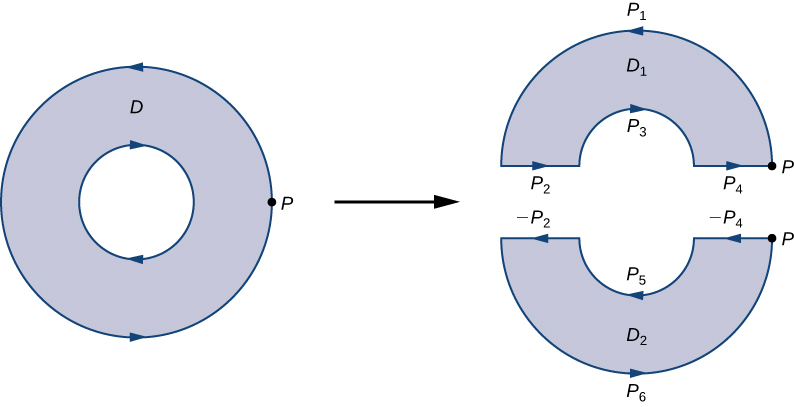
One thing to note is about orientation of the boundary. This is important when working with Green’s Theorem as it indicates whether to assign a positive or negative sign to the associated line integral. A positive orientaiton of $\partial S$ is the orientation (i.e. direction) that keeps S to the left (CCW) of $\partial S$ (the boundary) as one walks along it. So if we were to traverse the boundary of the region the opposite direction, our resulting line integral is opposite of what it would be if we were to traverse to the left. The thing I cannot wrap my head around till the time of writing is how the direction of the inner boundary is opposite of the outer boundary. Take a donut for instance, the outer boundary is traversed CCW meanwhile the inner boundary (inner-circle) is traversed CW as seen below:
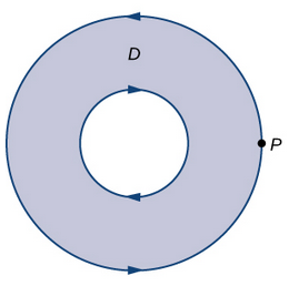
Taken from Libre Math. Illustrates how the inner and outer boundary are traversed in opposite direction but has positive orientation
The answer becomes obvious when you split the regions in half:
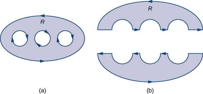
Here’s another example from Libretext that fully illustrates this:
The next major topic taught was surface integrals which calculates the amount of flux of a vector field passing through a surface. Those of you who have taken PHYS1002 or PHYS1004 or have a Physics background will know that a flux is the flow of some quantity such electric field lines or fluid mass that flows through a particular region per unit time. There are definitely some parallels with surface and path integrals in the sense that there are integral of scalar functions and also integrals of vector functions on orientable surfaces. But now we are integrating over surface rather than a path so we need to know how to parameterize a surface (i.e. decsribe a surface). In this course, we define a parameterization of the surface as the following:
Let a parameterization of a surface S in $\mathbb{R}^3$ be $G:U\subseteq \mathbb{R}^2 \to S\subseteq \mathbb{R}^3$
Once we know the parameterization of the surface, we can compute the surface area of S through the following equation:
Surface_Area(S) $= \int\int_U |\partial_u \vec{G} \times \partial_v \vec{G}|dA$
where u and v are independent variables of the parameterization which could be as simple as the variables x and y in cartesian coordinates or $\theta$ and $\varphi$ in spherical or cylindrical coordinates. In this course we say $dS = |\partial_u \vec{G} \times \partial_v \vec{G}|dA$. This may cause some confusion as outside literature states $dA = |\partial_u \vec{G} \times \partial_v \vec{G}|dudv$. They are equivalent statements but I just wanted to make that note.
Recall that the parameterization is a function that maps to $\mathbb{R}^3$ so taking a cross product between two $\mathbb{R}^3$ requires taking the determinant of a 3x3 matrix based on the following formula:
Cross Product using Determinant Formula: \(\vec{a}\times {b} = \Biggm\rvert\begin{bmatrix} i & j & k \\ a_1 & a_2 & a_3 \\ b_1 & b_2 & b_3 \end{bmatrix} \Biggm\lvert\)
If you are not used to the physics notation of i, j, and k, it’s essentially just our standard basis vectors $\vec{e_1}, \vec{e_2}, \vec{e_3}$ One key thing about taking the norm of a cross product is the ability to factor out common factors that are shared in a single row. This greatly confused me on how it works but I think that’ll be another blog post for another time since I’m very far behind my blog release schedule. For instance, we can factor out $R\sin\varphi$ from the 2nd row and $R$ from the third row in the following example:
\[\begin{align} \|\partial_\theta \vec{G} \times \partial_\varphi \vec{G}\| &= \Biggm\rvert\Biggm\rvert \begin{bmatrix} \vec{e_1} & \vec{e_2} & \vec{e_3} \\ -R\sin\varphi\sin\theta & R\sin\varphi\cos\theta & 0 \\ R\cos\varphi\cos\theta & R\cos\varphi\sin\theta & -R\sin\varphi \end{bmatrix} \Biggm\lvert\Biggm\lvert \nonumber\\ &= (R\sin\varphi)(R)\Biggm\rvert\Biggm\rvert\begin{bmatrix} \vec{e_1} & \vec{e_2} & \vec{e_3} \\ -\sin\theta & \cos\theta & 0 \\ \cos\varphi\cos\theta & \cos\varphi\sin\theta & -\sin\varphi \end{bmatrix} \Biggm\lvert\Biggm\lvert \nonumber \end{align}\nonumber\]However, the formula for the surface area only suffices when the scalar function we are integrating over is a constant function 1 (i.e. $\int\in S 1dS$). We need to introduce a new generalized equation to integrate scalar functions over surfaces:
Integrating Scalar Functions Over Surfaces: $\int\int_S fdS =\int\int_U f(\vec{G}(u, v))|\partial_u \vec{G} \times \partial_v \vec{G}| dA$
When taking the integral of vector functions over surfaces, we need to talk about the normal vector which again has been seen if you have taken an introduction to electromagnetism in first year.
normal vector: $\vec{n}$ is a normal unit vector to the surface meaning it has a magnitude of 1 and is perpendicular to the surface
The norm expresses the orientation of the surface. I like to think of the norm as describing the direction of the flux such as water where the norm is negative on the side at which the flux goes into the surface (inward) and positive when the flux leaves the surface (outward). I purged most of my Physics knowledge so I hope I am not saying something false. That’s the risk of writing about topics you don’t have much knowledge on I guess. Anyhow, for the purpose of this course, you ohave to choose the norm such that the norm is flowing outward which may require you to take the negation of the cross product $\partial_u\vec{G} \times \partial_v\vec{G}$.
Integrating a Vector Function Over a Surface: $\pm \int\int_U (\vec{F}\circ{G}\cdot (\partial_u\vec{G}\times\partial_v\vec{G})dA$
The final significant concept before Stokes Theorem is the discussion on curl and divergence. Divergence measures the amount of flux leaving at some point so if the divergence is negative, then the flux is converging instead of leaving. Curl as the name implies describes how particles at a point will rotate about the axis that points in the direction of the curl at the point. Notice the implicaton of the physical interpretation of divergence and curl. Divergence of a vector field measure a quantity which is a scalar value meanwhile curl describes how particles will behave and hence has both a direction and magnitude meaning the curl of a vector field is a vector.
More formally, let U be an open subset of $\mathbb{R}^n$ and $\vec{F}: U\to \mathbb{R}^n be a vector field of class $C^1$, then:
Div $\vec{F}$: $\nabla \cdot F = \partial_1 F_1 + … + \partial_n F_n$
curl $\vec{F}$ = $\nabla \times \vec{F}$
A trick to memorize the divergence and curl formula is to think the letter d from divergene as dot product and the letter c from curl as cross product. A neat trick I learned from a classmate and definitely helps remembering between the two. However, if you know the definition of divergence and curl, it should also be obvious as the dot product gives you a scalar value and a cross product gives you a vector. At the time I was taking the course, I did not know till I was writing about curl and diverge in this blog.
What isn’t surprisingly if that if the curl of a vector field is 0, it’s called irrotational. Similarly, when the divergence is 0, it’s called incompressible as the particles are neither convering or diverging from the point.
It turns out that divergence and curl can be used to describe Green’s Theorem:
Curl version: $\oint_C \vec{F}\cdot d\vec{r} = \int\int_D (curl \vec{F})\cdot \vec{k}dA$, $k$ is the unit bector in the z-direction
Divergence version: $\oint\vec{F}\cdot\vec{n}ds = \int\int_D div\vec{F}dA$
Anyhow, as we are talking about surface integrals, let’s talk about the analog for Green’s Theorem for surface integrals:
Divergence Theorem: Let $R \subset \mathbb{R}^3$ be a regular region with piecewise smooth boundary $\partial R$ (where $\partial R$ given an outward orientation). If the vector field $\vec{F}: R\to \mathbb{R}^3$ is $C^1$, then: $\int\int_{\partial R} \vec{F}\cdot \vec{n} dS = \int\int\int_R div\vec{F}dV = \int\int\int_R \vec{\nabla}\cdot F dV$
Now we reach the conclusion of the course and talk about Stokes’ Theorem. I did not know what Stokes Theorem was during the exam but let’s see if I can redeem myself right now:
Stokes’ Theorem: Let $S_o$ be a smooth surface with a piecewise smooth boundary $\partial S$ bounding $S\subseteq S_o$. Suppose $\vec{F}$ is a C’ vector field on S then:
$\int_{\partial S} \vec{F}\cdot d\vec{x} = \int\int_S (\vec{\nabla} \times \vec{F})\cdot \vec{n} dS$
I am not entirely sure how Stokes’ Theorem works still but the definition states that we have an oriented surface $S_o$ that contains S and hence the boundary of S, $\partial S$ is contained inside $S_o$. The surface is oriented by some normal vector field $\vec{n}$. What is often told is that Stokes’ Theorem is a generalization of Green’s Theorem for higher dimensions and that both Green’s Theorem and Divergence Theorem can be derived from Stokes’ Theorem. Green’s Theorem related a line integral to a double integral of a region so Stokes’ can be used to relate a line integral to a surface integral. Using this fact, the existence of $\partial S$ and the curl, we can attempt to make some sense to what Stokes’ Theorem is telling us. Recall the meme about Green’s Theorem tells us that the swirls inside the surface is equal to the big swirl along the boundary. We can view the swirls as the curl. So $\int_{\partial S} \vec{F}\cdot d\vec{x}$ represents the big swirl along the boundary while $\int\int_S (\vec{\nabla} \times \vec{F})\cdot \vec{n} dS$ represents all the little swirls on the surface. Whether this is an accurate depiction of Stokes’ Theorem is unknown to me. But that concludes the course description.
Review
Review: Starling is a great professor and is very considerate and reasonable. Personally I found the first half of the course much more interesting than the winter semester where we start talking about integration. In the fall semester, the talk about open balls and what it means for a set to be closed, path connected or convex were just more interesting than learning different techniques to integrate. The course heavily relies on you being familiar with first year calculus (MATH1052 and MATH2052). You do not need to be an expert in first year calculus but you do need to familiar with various concepts from the course. The course was fully in-person but Starling did try to be accodomating by recording the lectures and have a second version of the midterms for anyone who might be sick due to covid or for any other reason. Starling emphasized that if we were sick, we should not appear for the midterms because he’ll be accodomating. I know a few students who took this opportunity to recover. Unfortunately, not all professors were clear on how accodomating they would be so I know some students who looked very sick come for their midterms that were held on the same week for other courses but at least they got a break from writing the midterm for MATH2000. That was nice to see Starling be very considerate to the students. On the flip note, this means you will not be able to have access to your midterm papers nor the grades for your midterms till those who were unable to write their midterms complete the makeup midterms to minimize any potential unfair advantage the students may have. So you just have to be patient and wait for your grades which might matter to some students. I didn’t care too much since I already had an idea of how bad I did on the midterms. All I can say, studying a day before the midterms and exam is a terrible idea. Although Starling did record the lectures, he decided in the winter semester, he’ll just upload his lecture videos from previous years instead because the recordings from the fall semester were not that good quality.
Are there any proofs in the course? Yes there is. It is an honors course, so naturally there’ll be proofs. However, the amount of proofs on the assignments do decrease in the winter semester where it becomes more computational. Not saying there aren’t any proofs on the assignments in the winter semester, but there is definitely a noticeable decrease, at least that’s how I recalled it.
The course has 10 assignments, split evenly each semester. Meaning there were 5 assignments each semester worth 15% total I presume. To elaborate, all the assignments in the course were worth 30% so I presume, the assignments were split evenly between each semester. Unfortunately due to the TA strike during the winter semester, only 4 of the 5 assignments were marked. There were one midterm per semetser worth 10% each I presume. Both were done during class and were 1.5 hours each. The only grade distribution that was not equal from my understanding was the final exams for each semester. The midyear exam (the fall exam) was worth 20%. Meanwhile, the final exam (the winter exam) was worth 30%.
The great thing about Starling is that he has scanned notes online so you can either read the material ahead of time or read his notes to ensure you did not copy anything incorrectly. The scan notes and his notes on the board do differ but the general idea is the same. Starling has very good handwritting and he also knows how to make full use of the room such as the use of the chalkboard lights if one was available. This helps reading the board a lot. The same cannot be said about Mezo for MATH2100 but at least Mezo is a great lecturer as well.
In terms of the difficulty of the assignments, tests and exams, I cannot complain about them. Sure I did not do well on the tests and exams, it was because of my lack of studying. The questions on the tests and exams were perfectly reasonable. In fact, I think Starling was being nice to us on the final exam (the winter exam) and I just sat there feeling a bit bad. In terms of the assignments, there’s always one or two very tricky problem in the assigment. I often have to ask my friends or the TA for assistance to get through the tricky problems. Whether I asked my friends for help a lot in the winter semester is foggy in my mind even though it is more recent than the fall semester. I want to say I did but I honestly cannot recall. What I do know is asking for help a lot in MATH2100 assignments but that’s another course. So I might be confusing between the two courses. What I do recall was the assignments taking very long for me to complete because I was falling so behind in lectures during the winter. However, this is why the assignments are important. The only reason why I did not outright fail the midterm and final exams despite not studying enough is because I learned a lot from the assignments. Doing the assignments made me understand the lecture and tutorial materials much more. Talking about tutorials, the tutorials were sometimes very helpful for the assignments as it would sometimes be very similar to a problem on the assignment.
Is MATH2000 much harder than MATH1052 and MATH2052 is hard to say. I definitely would agree that the concepts of MATH2000 is much harder to grasp because it’s hard to visualize the concepts unlike in first year when things were in one-dimension. Sometimes, you just have to accept the definitions and theorems literally. I guess you could read the proofs but I stopped being a good student in 2nd year after I made the decision to drop my major (Physics) which broke both my motivation to study and every good habit I had as a student. Oddly enough, I have a transfer credit for MATH2004, so theoretically I should have an advantage in this course. But I recall nothing from the course as I didn’t have a great time in the course and I personally think the professor who taught me was bad at teaching (the professor is a good person and is funny but his teaching is not the best imo). But it could also be my mathematical maturity and appreciation was non-existent (I was a computer science major many years ago and if you know anything about the average CS kid, we hate math with a passion). Anyhow, not working in one-dimension did make me lost often times, especially during the winter semester.
Class size remained relatively the same in 2nd year, having around 60-70 students. But by the end of the semester, there was about 53 students according to OIRP. Let’s talk about course averages because why not? I have no clue if Starling is open for me to share course averages but I’ll give you a rough idea (i.e. not going to give you actual percentages):
- Fall Midterm: NA
- Midyear Exam: B
- Winter Midterm: D+
- Final Exam: C-
I suspect the fall midterm average is higher than the winter midterm average. However, this is pure speculation. I am guessing the average would be around a C- because I feel like students understood the material for the fall semester more than the winter. However, this is subjective. I know a lot of students had a hard time grasping open balls.
Before I try to speculate why the averages were what it is, it is best to break down how Starling formats his tests. The tests are 1.5 hours long and they typically have 5-7 questions with one bonus question. At least one question will be a true/false question where you need to state a reason why it’s true or give a counter-example if it’s false. These questions are quite tricky. In hindsight, when you discuss the answers with your fellow classmates, you realize the answer makes sense regardless if you got it or not unless no one got it. The exams are similar in length as their midterm counterpart and stlye where there is also a bonus question at the end of the exam. However, you are given 3 hours to write the exams. As neither the tests nor the exams are online, Starling will ask you to give the definition. A pattern I notice is that if he asks for the definition, he follows along with a second part in the question that relates to the definition. I believe I saw this on both midterms and on both final exams. So I won’t be surprised if you have something similar if you were to take MATH2000 with Starling which may not happen for a while since Starling is taking sabbatical and it’s either taught by Crann or Starling usually (unless Jaworksi is teaching the course). Starling’s winter semester exam did contain one question from the fall semester but Starling has provided us with a list of questions to work on relating to the fall semester and only one would appear word to word on the exam.
As stated earlier, I speculate the fall midterm average to be higher than the winter midterm average simply because of the material covered in the semester was easier to understand. Others may disagree which is fine. We are all wired differently so we find some concepts easier to understand than other. The issue with the winter semester was that you really needed a lot of practice and quite frankly, the material just does not click with me very well. Similarly to how integration in first year required practice to know which integration technique to use, the same idea applies to integration in higher dimensions. Unlike first year, there is actually a lot less integration techniques to recall than first year. There are just a lot more different types of integrals that you apply depending on how the question is setup. So it’s a bit deceiving to say there are a lot of new integration techniques you need to know and how to apply them. But it does not change the fact that the winter semester really requires you to practice a lot more to get a hang on how to set up the integrals. Computing the integrals after the integration has been set isn’t hard. The hardest part is setting up the integration with the correct bounds and the right coordinate system. I frankly did not have enough practice so I did not do so well on both the midterm and the final exam during the winter semester. The fall exam (midyear exam) was done quite well as reflected in the course average and my grade. I did extremely well on the exam obtaining an A+ from my memory. Starling gave us a sample midterm exam and that greatly helped boost the average even if it wasn’t the same. Combining our experience with the midterm and how the previous midterm exam was like, it gave us good preparation for the exam. The same does not seem to hold for the winter semester. Starling felt that there were no good previous winter midterm tests we could practice coupled with the fact you really need a decent amoun of practice doing integrals meant that the course did not fare well on the winter midterm. For the exam, Starling did give a previous winter exam to practice. But as the course was online, it probably wasn’t the best material to go off but it wasn’t too bad I would think. Starling also provided us previous exam questions that were given when Crann was professor for the course, and all I can say those were harder compared to what Starling would give. A speculation I have that supports my claim that the winter semester is harder is the fact that the final exam for the winter semester is worth more than the midyear (fall) exam by 10%.
The SAT option given to us because of TA strike may have influenced our decisions to study on the final exam. But I think most of us still opted to use that as a last resort because I would think the vast majority of us wanted to do decently on the final exam because we need to ensure we have a decent understanding of the material for future courses. In addition, there is a minimum grade requirement if one was in the pure math stream or planning to take MATH3001: Real 1 for fun like me. I mean my entire academic career studying Math is for fun anyways. And I am sure most of us in the Math honors program are in Math because we want to study Math so I doubt the SAT option had much influence in how much we were going to study for the exam.
Overall, the course was good but I wished I took my studies more seriously. There are definitely a lot of gaps in my knowledge in the course and I messed up big time on the final exam. While I do not think my failure to understand the winter semester material will negatively impact my ability to do my future courses seriously, I do feel a bit upset to myself that I had another opportunity to learn multivariable calculus and I blew it. I definitely understand the material much more now than I did 6-7 years ago but it is not to the level I would be satisfied with. Also rip my CGPA but I guess that’s what you get when you slack off.
Credits:
- MATH2000 Notes From Charles Starling
- MAT237 Notes from Tyler Holden
- Notes I found online. Never taken a course with Tyler Holden but I heard he is a great prof from classmates who have taken courses with him
- MAT237 Lecture Notes 2018-2019
- A link I randomly stumbled upon when trying to figure out what zero content was. These notes heavily follow Folland’s textbook.