This is a course review of MATH1800 - Introduction to Mathematical Reasoning taken at CarletonU in winter 2023. The lectures were synchronous and quizzes was where the weekly quizzes were held. This review is going to be very biased as this is “technically” my 3rd time taking this course. I first took an introductory course to Mathematical proofs over 7 years in 2015 when I first began my studies in Computer Science. This is the first course that introduces you to the world of Mathematics that is very different from the math I have been taught in my entire life and was one of the few courses that later pushed me into Mathematics despite almost failing this course at my alma mater by 1%. Read the long course description section below to read more about my thought and experience of the material of the course.
TLDR:
- Mathematical proofs is very different from your usual math in Highschool and even for Math in Engineering
- Crucial course for anyone who has an interest in Mathematics
- Practice and review the content regularly, proofs takes a while for your brain to register and get used to
The review is split into 2 main parts:
- Long Course Description: In-depth talk about the course topic from how I understood it
- Course Review: Solely focuses on the teaching style, difficulty, and anything that would be of interest
Professor: Daniel Panario
Course Delivery: Synchronous lectures with synchronous tutorials
Class Size: 50 students (March 28 2023)OIRP
Course Description (from website): Elementary logic, propositional and predicate calculus, quantifiers, sets and functions, bijections and elementary counting, the concept of infinity, relations, well ordering and induction. The practice of mathematical proof in elementary number theory and combinatorics.
CLICK HERE TO SEE JUST THE COURSE REVIEW
Course Description (LONG) with Commentary:
The course begins with an introduction to sets which may or may not be a review and is probably reviewed again in Calculus for general math
students (at least it was when I was studying Computer Science).
Sets as you probably already know is a collection of objects where the objects are called elements or members of the set.
It’s similar to an array in programming where members in the array are called elements.
However, the difference is that elements in the sets are unique while in an array, they are not.
Similarly to how an empty array in C is denoted as {} and empty set in Mathematics is denoted as $\emptyset = \{\}$.
Another parallel to programming is how { {} } is not the same as {}.
In baby set theory, $\emptyset$ and $\{\emptyset\}$ are not the same as $\{\emptyset\}$ has one element while $\emptyset$ has no elements in the set. Various basic set notations are introduced such as what the following means: $\in, \notin, \subset$. In addition to covering set notations, the course also covers common sets in Mathematics such as the irrational and rational sets.
Something new in the first topic is the idea of cardinality, denoted as $|S|$ is the number of elements in a set. A new set inroduced to students is the power set:
Power Set: $P(A)$ the set containing all subsets of a set A Example: A = {1, 2} $P(A) = \{\emptyset, \{1\}, \{2\}, \{1,2\}\}$
The course then delves deeper into sets by describing the operations that can be done to sets such as union, intersection, difference, and what does the complement mean. ALl of these ideas were introduced to students before University most likely but never formally defined. The course does not start with anything difficult as students have been dealing with sets since elementary school, at least that’s what I can recall. While the ideas covered are simple, they do require practice to distinguish between elements and sets. For instance, I can see students making the following mistakes:
- $\{1\} \in \{1, 2, 3\}$ WRONG
- $\{2\} \in \{1,\{1, 2\}\}$ WRONG
- having trouble to write down the set for $P(\{\emptyset, \{\emptyset\}\})$
- $A = \{\{1, 2\}\} = 2$ WRONG
- $A = |\{0,2,4,…,10\}| = 5$ WRONG (it’s actually 6 because you need to include 0 when you are counting)
- $|A \cup B| = |A| + |B|$ WRONG
To answer the last question, one must understand the Principle of Inclusion and Exclusion. This is the hardest concept to wrap your mind around and answer. Problems relating to Principle of Inclusion and Exclusion can be quite tricky to answer which you will see if you take the course. To understand why $|A \cup B| = |A| + |B|$ is wrong, it helps to draw a diagram. You will realize you counted $A\cap B$ twice. I encourage you to draw the diagram and see for yourself why and also to find the statement for three finite sets to truly understand the principle of inclusion and exclusion.
The next topic in the course is logical connectives. Before we can start talking about logical connectives, we first need to began with what a statement or proposition is as logical connectives connects between one or more statements to form compound statements. A statement is a declarative sentence that is either true or false (but not both). If you are familiar with programming, this should be familiar to you. Although this may sound quite obvious, it is of great importance that students know what is and more importantly what is not a statement. A mathematical proof is a compound of statements just like how a program is a stack of statements (instructions). Logical connectives allows one to construct more complicated statements. Logical connectives are not solely binary but can also be unary as well. For instance, the negation of a statement $P$ (i.e. the not operator in CS) causes the statement to have the opposite truth value. Negation is denoted as either $~P$ or $\neg P$.
Another parallelism to Computer science is the usage of truth table that one might be familiar with if they ever explored digital systems (i.e. logic gates). In fact, you could think of logical connectives as logic gates. We have Disjunction i.e. OR (syntax: v) and conjunction i.e. AND (syntax: $\land$). In this course, the basic 3 logical operators: AND, OR, and NEGATION can create any other logical connectives covered in the course such as exclusive or $\oplus$ as $(P \ V \ Q) \land \neg (P \land Q)$. The first concept that bothered me for more than a few minutes was the implication truth table. The implication statement (i.e. $P \implies Q$) as one would expect is simply in plain English as If P, then Q. How I interpreted as a programmer is: If P is True, then do Q which isn’t an implication/conditional statement in Mathematics.
Suppose P and Q are statements:
| P | Q | $P \implies Q$ |
|---|---|---|
| F | F | T |
| F | T | T |
T |
F |
F |
| T | T | T |
Note: The way I wrote my truth table might irk TAs because they love to begin with every plain statement to be true and work their way to making every plain statement to be false at the bottom
When I first saw this truth table in this course, my mind broke. I was totally not expecting that the implication can still be true when P is false. My brain is wired to think about whether or not the if statement would be evaluated and did not conceive that implication and if statements are two different logical operators. What the truth table highlights is that there is only one case where the implication fails, that is when P is true but Q is false, then the statement is false. For instance, if I claim that if I am elected, I will lower taxes but do not do so despite being elected, I broke my promise. Hence, the implication is false. Let’s look at the case when Q is not true but the implication is still true. The following statement: 1 + 1 = 3 then 1 + 1 = 2 is a true statement despite 1 + 1 does not equal to 2 but rather 3 (if we are operating in the reals with normal addition). This is a weird statement that I find it hard to wrap my mind still.
Some interesting terminology covered in the realm of logic are tautology and contradiction. Contradiction is a compound statement that is always false which isn’t too surprising. Tautology is the opposite of contradiction where the compound statement always evaluate to be true. Although the term mighht not be interesting, it was the first crack I started to notice in my knowledge of mathematical proofs when I entered 2nd year not taking MATH1800. In MATH2000, I was so lost when my TA mentioned this word and my classmates were looking at me weirdly because it was a term covered in MATH1800. Though not significant, the cracks of my knowledge started to be more apparent throughout my fall semester of 2nd year which I might go into as I continue writing this long description of what the course covered.
The last part of this chapter talking about logics are quantifiers. I am not sure how to describe quantifiers aside from they are something that they convert an open sentence into a statement and have some relation to the idea of quantity. There are only two quantifiers to consider:
- universal ($\forall$)
- existence ($\exists$)
Quantifiers are always seen in statements that consider a domain (i.e. a set of values). For instance, $\forall x \in S, P(x)$ can be translated as “for every x in the set S, the statement P(x) is true”. While, $\exists x \in S, P(x)$ can be translated as “there exists an x in the set S that the statement is true”. The difference between the two is akin to the difference between an AND statement and an OR statement:
$P(x_1) \land P(x_2) \land … \land P(x_n)$
v.s
$P(x_1) \ V \ P(x_2) \ V \ … \ V \ P(x_n) $
Here’s an example of a statement that uses a qualifier: $\forall x\in\mathbb{R}, x^2 \ge 0$
The only tricky part of quantifiers is to make use of De Morgan’s Law for Quantifiers because you need to realize how to negate substatements that does not change the meaning of the original statement.
The third section of the course covers proof techniques that are not recursive such as direct proofs and contrapositive. These two proof techniques along with contradiction are very important to know to survive most of the proofs covered in other Mathematics courses aside from statements that are recursive. A lot of problems in this section involves solving problems involves parity (i.e. even or odd) such as the statement: If n is odd then 5n+9 is even. It is fundamental to know the definition of even and odd to solve any types of problems that involves parity.
Even: An integer $n$ is even if $\exists k\in\mathbb{Z}$ such that $n = 2k$ which is to say that an integer $n$ is even if it’s divisible by 2
Odd: An integer $n$ is odd if $\exists k\in\mathbb{Z}$ such that $ n= 2k + 1$ which is to say that an integer $n$ is odd if it’s not divisible by 2
Direct proof as the name implies is straightforward technique whereby you assume the premise P(x) is true and try to show the statement Q(x) must also be true. Direct proof is the most simplest method to prove a statement but is not suitable for all types of problems. Hence why proof by contrapositive is taught. Often times, there are problems where it would be hard to prove in the forward direction but if we were to approach the problem in the other direction, it would be much simpler. Direct proofs are in the form of $P(x) \implies Q(x)$ but contrapositive approaches the problem $\neg Q(x) \implies \neg P(x)$. Essentially, contrapositive is another way of looking and approaching the same problem but in a different angle. Although tempting, you cannot approach the problem supposing $Q(x)$ and prove for $P(x)$ (i.e. $Q(x) \implies P(x)$). The statement might not remain true unless the problem is biconditional (i.e. $P(x)\iff Q(x)$). Having a good understanding of how direct, contradiction, and contrapositive proofs work is essential not only succeeding in MATH1800 but in your entire Mathematical Career as you will be required to know how to approach Mathematical proofs if you decide to go into Mathematics.
Throughout the course so far, we have only been tackling problems that did not have different cases. For instance, if the parity (eveness) of a number is important, the statement would have explicitly stated this i.e. if $x$ is an even number, then __ . Often times, a statement can be true regardless of parity which can complicate the proof if one was to tackle both cases simulatenously. That is where proof by cases becomes useful. Proof by cases as the name implies breaks down a problem into several different manageable cases. For instance, if we get a statement $P(n)$ that applies for both even and odd natural numbers, then there are two cases to consider. Therefore, separating the cases into two will not only be sensible but it will be easier on the mind as you can forget the other cases temporarily as you tackle each case separately. An example of this shown in lecture is the following:
\[\text{Let } n\in\mathbb{Z}. \text{Then } n^2 - 3n + 9 \text{ is odd} \nonumber\]From the statement above, you can see that $n$ can be both even or odd as no restriction was applied to $n$ aside from $n$ being an integer.
The next section of the course discusses about divisibility. I once foolishly stated to a class that divisibility will never be seen again from their core courses in their program and I shortly regretted this statement. As a former student of computer science, the topic of divisibility is rarely discussed in their senior courses aside from computer science electives such as cryptography. I did not realize how important divisibility was in the Mathematics program as it appears often in group theory. The topic of divisibility is discussed both in MATH1800 and in MATH1152 so students should be expected to already have some prior knowledge of divisibility. Regardless, the definition of divisibility is once again introduced for students outside of the Mathematics program. The notation and English for divides does confuse me once in a while but it does make sense.
Let $a,b \in \mathbb{Z}, a\ne 0$. $a$ divides $b$ (written as $a | b$) iff $\exists c\in\mathbb{Z}$ such that $b = ac$
We say that $b$ is a multiple of a and that $a$ is a divisor of $b$
If $a$ does not divide $b$, we write $a \not|\; b$
For instance, $3 | 6$ because $6 = 3\cdot 2$ but $4 \not|\; 6$ because there does not exist an integer c with $6 = 4c$. This entire section on divisibility goes through a lot of properties of divisibility that is neat and at least to me is an introduction to number theory (disclaimer: I have never taken number theory, so that is just my naive view of number theory).
Recall how remainders are the “left overs” after performing a division when numbers do not divide nicely. Every integer can be expressed as a multiple of a number plus some remainder. For instance, every integer can be expressed as 2q or 2q+1 where the possible remainders are just 0 and 1 where q is some integer. Similarly, every integer can also be expressed as one of 3q, 3q+1, 3q+2. When working on solving proofs involving divisibility, proof by cases can be very helpful since we may need to consider different cases involving remainders. For instance, the following problem can take advantage of proof by cases and proof by contrapositive:
\[\text{Let } x\in\mathbb{Z}. \text{If } 3\not|\; (x^2-1), \text{then } 3 | x \nonumber\]As the forward direction would be hard to tackle, by contrapositive, we can suppose instead $3\hspace{-4pt}\not| x$ and show $3 | (x^2-1)$ instead. As $3\hspace{-4pt}\not| x$, there are two cases to consider: when the remain is 1 or when the remainder is 2 i.e. $x = 3q+1$ or $x = 3q+2$ where $q\in\mathbb{Z}$. The next important idea for divisibility is congruence which is another word for equivalent (do not get confused between equality and equivalence as the former means similar which should be familiar from geometry).
For $a,b \in\mathbb{Z}$ and $n\in\mathbb{N}, n\ge 2$, we say a is congruent to b modulo n, $a \equiv b \pmod{n}, \iff n|(a-b)$
An example is $15\equiv 1\pmod{7}$ since $7|(15-1)$ but $15\not\equiv 2\pmod{7}$ as $7\hspace{-4pt}\not|(15-2)$. The topic of modulo and congruence introduces to modulo arithmetic which does take some time to get used to. One thing I would like to highlight from the lecture is the various ways to represent modular arithmetic:
\[\begin{align*} a \equiv \pmod{n} & \iff n|(a-b) \nonumber \\ & \iff a - b = kn \text{ for } k\in\mathbb{Z}\nonumber \\ & \iff a = b + kn \text{ for } k\in\mathbb{Z}\nonumber \end{align*}\]The next section revisits the topic of sets. Now that we are equipped with knowledge of basic mathematical proofs, we can now tackle problems relating to sets which is either the hardest or second hardest type of problems to prove in the course, the other being counting problems. To solve problems relating to sets, you have to rewrire how you think (though this entire course forces you to rewire how you approach and think about problems in general). Questions in this topic usually relates to showing two sets being either a subset or equal to the other set. The basic premise to show a set A is a subset of B, $A \subseteq B$ is to show for any arbitrary $x\in A$ that it is also in B, $x\in B$. Meanwhile to show equality, you need to show that both sets are subsets of each other i.e. $A\subseteq B$ and $B\subseteq A$. Knowing that two sets are equality if they are subset of each other, it is more worthwhile to discuss how to show a set is a subset of another set.
Unlike previous types of problems in the course, problems relating to sets have a lot of logics and words required in the proof. The reason why I think this topic contains the hardest types of problem is that I am wired to think of Mathematics as arithmetic algebra where I just need to know how to manipulate numbers and variables. However, when dealing with sets, we need to fundamentally understand our basic definitions and try to be as verbose as we can so that we can convey our thoughts properly and logically. Let’s go through an example to see what I mean:
\[\text{For any sets } A \text{ and } B, \overline{A\cap B} = \bar{A} \cup \bar{B}\nonumber\]As this problem is trying to show equality, we immediately know we need to show $\overline{A\cap B} \subseteq \bar{A} \cup \bar{B}$ and $\bar{A}\cup \bar{B} \subseteq \overline{A\cap B}$. One may immediately recognize this is an immediate consequences from DeMorgan’s Law. However, we need to prove the statement using DeMorgan’s Law.
To begin, we first show the forward direction: $\overline{A\cap B} \subseteq \overline{A} \cup \overline{B}$
Let $x\in \overline{A\cap B}$. Then we have $x\notin A\cap B$. Here is where things get weird. It is tempting for myself to think $x\notin A\cap B \implies x \notin A$ and $x \notin B$ but this statement is FALSE. Even after I completed the course, my mind is still stuck thinking the statement is true. Good thing TAs and professors cannot read your mind when they are reading your proofs because I memorized the structure of how the professor answers these types of questions. So I got away thinking the statement was true. It’s hard to conceptualize why the statement: $x\notin A\cap B \implies x \notin A$ and $x \notin B$ is FALSE, so diagrams will help a lot:
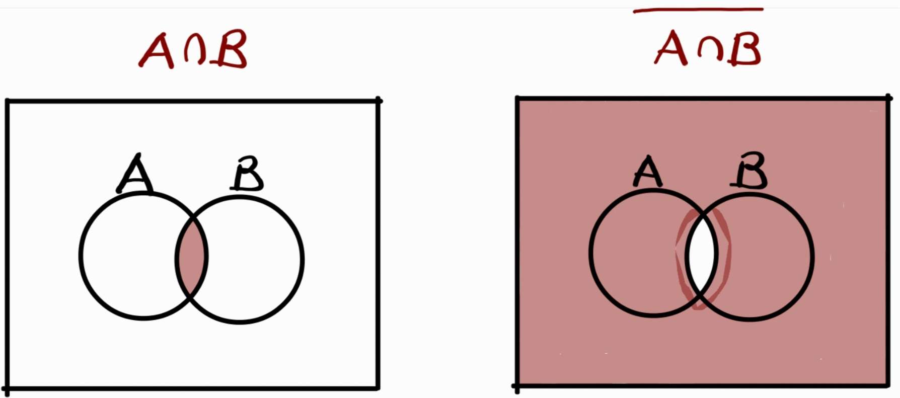
$x\notin A\cap B does not mean x cannot be in either A or B. It can lie either in A or B or outside of A and B as long as it's outside the intersection
From the diagram above, one can see why the statement is false. As long as x is not in the intersection of A & B, it can lie anywhere in the “universe” including in A or in B. I do not know why I struggled to conceptualize this as it is quite obvious when you draw the diagram or think of the end goal of the proof. How I survived and performed very well in the course was to remember to write the following logic:
So it is not the case that $x\in A$ and $x\in B$. By DeMorgan’s Law, $x\notin A$ or $x\notin B$
I do not know why but the statement: It is not the case that is what confuses my brain. However, this is DeMorgan’s Law in a nutshell but with more words than I am more comfortable with. To conclude the forward direction, we can see that $x\in \bar{A}$ or $x\in\bar{B}$. This implies $x\in\bar{A}\cup\bar{B}$. The reverse direction is similar and is left as an excercise to the reader :P
According to the lecture notes, the next topic is proof by contradiction which I thought was already covered when direct proof and proof by contrapositive was introduced. The basic idea of proof by contradiction is to assume the premise is false and derive a contradiction. Proof by contradiction is a very powerful tool that I find myself using a lot in my other courses. Oddly enough, I tend to not use proof by contrapositive aside from true and false questions but instead use proof by contradiction outside of the course. Proof by contrapositive is definitely a useful tool as we saw in the beginning of the course but when working on problems that are not algebraic in nature (i.e. manipulating variables and numbers), I typically find proof by contradiction to click in my brain more easily. Proof by contrapositive is great in truth and false problems because there are times when a statement is obviously true based on a proven theorem or lemma that we are forced to remember for the midterms and exams. But when I do not know how to approach a proof, my first instinct is to prove what would happen if the statement was false.
A sample problem where proof by contradiction is great is:
- There is no smallest positive real number
- The sum of a rational number and an irrational number is irrational
- If a is even and b is odd, then $4 \hspace{-4pt}\not |(a^2+2b^2)$
- in this scenario, you assume a is even and b is odd still but now you suppose $4 |(a^2+2b^2)$
- $\sqrt{2}$ is irrational
The next topic is existential proofs but I’ll omit discussing about this topic as there isn’t anything notable I want to say about this topic.
The next topic is arguably the most important proof technique for Computer Science, induction. Induction is the framework or the Mathematical logic that allows programmers to write recursive functions. Recursive functions are extremely important topic in Computer Science.
While the usage of recursion may be banned in critical safety software, recursion allows elegant solutions and simple code to problems that would otherwise be very ugly and confusing if one was to use an iteration instead. The argument against recursion is not due to any flaw in the mathematical concept itself but rather how dangerous recursion can be if it is not bounded and properly written, aka the stack overflows. Recursion is used in all types of software used in non-critical software including your operating system, at least at some point of time it did if it does not exist anymore.
Mathematical Induction is used to prove statements that are always true regardless of the input (for all numbers greater or equal to the smallest case) and not just true only for a specific natural number only.
Principle of Mathematical Induction
Let P(m) be a statement for each integer $n\ge m$. If
- P(m) is true
- the implication: if P(k), then P(k+1) is true for every integer $k \ge m$
then P(n) is true for every integer $n\ge m$
Mathematical Induction involves three main steps:
- Base Case: Prove the statement P(m) is true
- Induction Hypothesis: Assume the statement P(k) is true for $k\ge m$
- Induction Step: Showing the statement is true for the next number k+1. In the proof, we need to utilize the induction hypothesis, P(k), directly to help us arrive to the proof
An example of a type of question where induction can be used is the following:
For $n\in \mathbb{N}, 1+2+3+…+n=\frac{n(n+1)}{2}$
The base case would be to prove for $P(1) = 1 $ and $P(1) = \frac{1(1+1)}{2} = 1$
The induction hypothesis would be to suppose the statement $1 + 2 + … + k = \frac{k(k+1)}{2}$ holds for $k\in\mathbb{N}$
The inductive step is to show the statement is true for $P(k+1) = \frac{k(k+1)}{2}$. The key to solve problems using induction is to write down what our starting and ending goal are. This applies to every single proof as well.
Our end goal is $P(k+1) = \frac{(k+1)(k+2)}{2}$ and we start with:
\[\begin{align*} (1 + 2 + 3 + ... + k) + k + 1 &= \frac{k(k+1)}{2} + (k + 1) \tag{induction hypthesis} \\ &= (k+1)(\frac{k}{2} + 1) \tag{factor out k+1} \\ &= (k+1)(\frac{k}{2} + \frac{2}{2}) \\ &= (k+1)(\frac{k+2}{2}) \\ &= \frac{(k+1)(k+2)}{2} \end{align*}\]By the principle of Mathematical Induction, the results holds for $\forall n\in\mathbb{N}$
While this example is quite simple, you do need to be good at manipulating numbers and know your basic algebra to arrive to your final answer. Induction problems can get hard when you need to consider more than one case but this is not heavily tested in MATH1800 but do not be surprised if you do enounter one, especially in your upper year courses. In addition, there are problems that are hard to solve if you do not realize the base case can be utilized in the proof, especially when the statement involves inequalities. The following problem illustrates very well these two points: For all integers $n\ge 5, 2^n > n^2$. In the inductive step we have the following:
\[\begin{align*} 2^{k+1} &= 2 \cdot 2^k \tag{power laws} \\ &> 2 k^2 \tag{inductive hypothesis} \\ &= k^2 + k^2 \tag{basic algebra}\\ &= k^2 + k\cdot k \tag{more basic manipulation} \\ \end{align*}\]But this is where most students will stumble. It is not obvious how we can go from $k^2+k\cdot k$ to our final goal $(k+1)^2$. It does seem we are on the right track because we have a 2 degree polynomial but we cannot simply jump to our end goal as we need to somehow show $2k^2 > (k+1)^2$. This is where our base case comes in handy. We know that $k\ge 5$ so we can substitute $k=5$:
\[\begin{align*} 2^{k+1} &> k^2 + k\cdot k \\ & \ge k^2 + (5)k \tag{since $k\ge 5$}\\ & = k^2 + 2k + 3k \\ & \ge k^2 + 2k + 3(5) \tag{since $k\ge 5$}\\ & > k^2 + 2k + 1 \\ & = (k+1)^2 \end{align*}\]When I first saw this problem, I was amazed how much manipulation was required and it reminded me of problems I used to solve many years ago in my theoretical computer science courses in 2nd year where we had to solve a lot of problems similar to these. So it was a nice experience that I had little trouble solving these problems compared to when I was a young lad who hated Math.
There is another form of induction called Strong Induction which is similar in structure and approach with one key difference, regular induction assumes the property holds for k, meanwhile in strong induction, we assume the property holds for everything from the base case up to k
Strong Induction Hypothesis and Inductive Step: assume P(i) for every i with $\mathbf{m \ge i \ge k}$, then prove for for P(k+1) for $k\ge m$
Strong induction is great for solving problems that have recurrence relations such as sequences because of their structure to rely on previous terms. A classical example to visualize induction is to think of a series of dominoes lined up. If the previous dominoes fell, then the next domino must also fall is the idea of induction.
The next set of problems introduced in the course are interesting. The lecture is titled “Prove or Disprove” and as the name implies, the course now introduces problems that maybe true or false. So far in the course, we’ve only been trying to solve problems that we are told is true. However, in Mathematics we do not always know if a statement is true or false. It is our job to figure out whether a statement is true. So this is our first introduction to getting an intuitive and logical sense whether a statement is true or not. The general idea is that we should always try to see if the statement holds for some simple set of numbers and if it seems to hold, then we try to prove the statement. If the statement turns out to be false during our attempt to prove the statement, then we get an insight as to why the statement is false. It only takes one counterexample to disprove an entire statement.
The next few sets of lectures are talking about relations, equivalence classes, and functions. Relations are interesting because it is something we should know but maybe don’t have a complete picture of. This was also my first time seeing how relations are defined formerly (I may have been taught this in the past but I sure don’t recall it).
Relations: for sets A and B, a relation R from A to B is a subset of the set {(a,b): $a\in A$ and $b\in B$}
If $(a,b)\in R$, we say a is related to b by R and noted as $a R b$
This is where domain, image, and inverse is reintroduced:
Domain: dom(R) $= \{a\in A: (a,b)\in R$ for some $b\in B \}$
Range: range(R) $= \{b \in B: (a,b)\in R$ for some $a\in A\}$
Inverse Relation: $R^{-1} = \{(b,a): (a,b)\in R\}$
Let’s look at an example: $A = \{a,b,c\}, B=\{1,2,3\}$ and $R=\{(a,1),(a,3),(b,2),(b,3)\}$
dom(R) = {a,b}
range(R) = {1,2,3}
$R^{-1} = \{(1,a),(3,a),(2,b),(3,b)\}$
Properties of relations are also discussed in the course which is something I have seen before:
Reflexive: R is reflexibve if $\forall x\in A, x R x$
Symmetric: R is symmetric if $\forall x,y \in A, x R y \implies y R x$
Transitive: R is transitive if $\forall x,y,z\in A,$ $(x R y \land y R z) \implies x R z$
The third property is interesting to me because it is a property I love to use. A simple example is if $a > b$ and $b > c$ then by transitivity, $a > c$ In this section, you’ll be give a bunch of relations and you’ll need to see what properties the relations satisfy and which one breaks.
The next topic is on Equivalence Relations which are essentially relations that satisfy all 3 properties: reflexive, symmetric, and transitive. An equivalence class is a subset of a set A who is related by an equivalence relation with a specific element.
Equivalence Class: for $a\in A$, the set $[a] = \{x\in A: x R a\}$ is an equivalence class.
The types of problems presented in class are not difficult but require one to be viligant because it is easy to make a mistake. One also needs to be able to redefine the condition in different ways. For instance, if we were trying to define an equivalence class an odd number a for a relation R on $\mathbb{Z}$ defined by $a R b$ if $5a + b$ is even:
\[\begin{align*} [a] &= \{x \in \mathbb{Z}: x R a \} \\ &= \{x \in \mathbb{Z}: 5x + a \text{ is even} \} \\ &= \{x \in \mathbb{Z}: 5x \text{ is odd } \} \\ &= \{x \in \mathbb{Z}: \text{ x is odd } \} \end{align*}\]The ability to break down the condition on a relation to its most basic and simplest for does take some practice as usual. There are theroems about equivalence class and residue classes discussed in this section as well. I’m going to skip that to talk about functions very briefly, as in state a bunch of definitions and move onto counting problems.
Function: $f: A\to B$ is a relation from A to B where every element of A is the first coordinate of exactly one ordered pair in f
dom(f) = A
codomain(f) = B
image of a: f(a) = b where $a\in A$ and $b\in B$
range(f) = $\{b\in B: (a,b)\in f$ for some $a\in A\} = \{f(a): a \in A\}$
Image of A: f(A) = range(f)
Inverse Image: or Preimage: of a set D is $f^{-1}(D) = \{a\in A: f(a)\in D\}$
$B^A$: for non emptysets A and B, $B^A$ is the set of all functions from A to B
$|B^A| = |B|^{|A|}$
Injective: $f: A\to B$ is injective if $\forall x,y \in A, f(x) = f(y) \implies x = y$ $|A| \le |B|$ if $f:A\to B$ is injective
Injective (counterpositive): $f: A\to B$ is injective if $\forall x,y \in A, x \ne y \implies f(x) \ne f(y)$
Surjective: $f: A\to B$ is surjective if for each $y\in B \ \exists \ x\in A$ such that $f(x) = y$ If A and B are finite sets and $f:A\to B$ is surjective then $|A|\ge|B|$
Composite Function: $(g\circ f)(n) = g(f(n))$
If $f: A\to B$ and $g:B\to C$ be functions
- if f and g are injective, then so is $g\circ f$
- if g and g are surjective, then so is $g\circ f$
- if f and g are bijective, then so is $g\circ f$
Inverse Functions: for $f:A\to B, (f^{-1}\circ f)(x) = x \in A$ and $(f\circ f^{-1})(y) = y \in B$ f must be bijective for an inverse to exists
Note: Preimage and Inverse Functions are two different things!!! Reciprocal and Inverse are also two different things!!! Preimage of a set C under a function f is the set of all elements that map to elements in C through f Inverse function of a function f “undoes” the action of f, obtaining the original input
Example: Find an inverse of a bijective function $f:\mathbb{R}-\{\frac{-2}{3}\}\to \mathbb{R}- \{\frac{2}{3}\}$ defined by $f(x) = \frac{2x+3}{3x+2}$
Since $(f\circ f^{-1})(x) = x$ for all $x\in \mathbb{R}-\{1\}$, we have
\[\begin{align*} x = f(f^{-1}(x)) &= \frac{2(f^{-1}(x)) + 3}{3(f^{-1}(x) )+ 2} \\ x(3f^{-1}(x) + 2) &= 2f^{-1}(x) + 3 \\ 3xf^{-1}(x) + 2x &= 2f^{-1}(x) + 3 \\ 3xf^{-1}(x) - 2f^{-1}(x) &= 3 - 2x \\ (f^{-1}(x))(3x - 2) &= 3 - 2x \\ f^{-1}(x) &= \frac{3-2x}{3x-2} \end{align*}\]To check,
\[\require{cancel} \begin{align*} (f\circ f^{-1})(x) &= f(\frac{3-2x}{3x-2}) \\ &= \frac{2(\frac{3-2x}{3x-2})+3}{3(\frac{3-2x}{3x-2})+2} \\ &= (\frac{6-4x}{3x-2}+ 3)(\frac{9-6x}{3x-2} + 2)^{-1} \\ &= (\frac{6-4x}{3x-2}+ \frac{3(3x-2)}{3x-2})(\frac{9-6x}{3x-2} + \frac{2(3x-2)}{3x-2})^{-1} \\ &= (\frac{5x}{\cancel{3x-2}})(\frac{5}{\cancel{3x-2}})^{-1} \\ &= \frac{\cancel{5}x}{\cancel{5}} \\ &= x \tag{as required} \end{align*}\]The course ends with counting problems, the problems I hate the most. These types of problems may be familiar if you have done a probability course. These types of problems ask you how many ways can you arrange a set of some item, how many combinations are there for … and etc.
The first topic is the product rule which can be used to figure out how many possible ways are there by simply multiplying all the possible ways:
Example: First and last initials consists of two letters. How many possible two letter initials are there? What about if we do not allow repeated letters?
There are 26 letters to choose for the first initial and there are 26 letters for the 2nd initial, so there are $26^2$ possible initials
If we do not allow repeated letters, then there are 26 letters to choose from for the first initial but only 25 letters that can be choosed since the previous initial consumed one letter. Hence there are $26 \cdot 25$ possible initials.
The next topic is my most favorite principle in the course, the Pigeonhole Principle. This blew my mind years ago when I was first introduced this concept.
Pigeonhole Principle: Let $k\in \mathbb{N}$. If k+1 or more objects are placed into k boxes, then at least one box contains two or more objects
This principle is so simple yet so powerful. Take the course to see what it is about or read up about it online because it’s such a powerful tool.
The course ends with permutatins and combinations. The difference between permutations and combinations is that permutations cares about the ordering of the objects while combination do not. What is interesting is that you can derive permutation from the product rule which was neat to see.
Permutation: If $r \le n$, then $P(n,r) = \frac{n!}{(n-r)!}$
Combination: If $ r\le n$, then $C(n,r) = \frac{n!}{r!(n-r)!}$
I will not go into combintorial proofs in depth as I am terrible solving problems relating to counting. But I will likely be talking about combintorial proofs and counting problems in the future either when I talk about a third year discrete mathematics course or in a probability course review.
Review
Review:
MATH1800 is an introductory to Mathematical Proofs and is a foundational course that all Math majors must take to be successful in their academic career in Mathematics. I decided in first year that I could skip this course as I have a transfer credit and technically this would have been my 3rd time taking the course if I had to take it again at CarletonU. While I did very well in first year and doubt retaking MATH1800 would help me get better grades in first year, I now feel that I truly missed out an integral part of the experience of being a Math student. This course likely is the first course that students are exposed to Mathematical Proofs as the Math from Highschool does not reflect the true experience of Mathematics as a subject. Mathematical Proofs is not only the foundation of the subject itself, it helps wire your brain to think and approach problems in a different way. I know when I was first exposed to Mathematical Proofs 8 years ago, it broke my brain because I could not comprehend what I was seeing. Being a Computer Science student at the time and fresh out of Highschool, I thought Math was boring and was a series of seeing patterns and memorizing steps. However, Math is more than seeing patterns and memorizing equations and steps to solve problems, it’s an “art” that is very sophiscated and deep. The Highschool experience is a deceit and a lie of what Math truly is. The course I took many years ago is one of the many reasons why I decided to quit my job and revisit Mathematics. I think this course will make you truly appreciate and have a taste of what Mathematics is regardless if you are in the Mathematics program or not.
Panario is very approachable professor and is quite lively for a Math professor (Bretts Stevens is on a different level though). The lectures were enjoyable and I like how Panario went over the proofs and examples. The course has slides which is a life saver because you don’t have to take notes and just focus on the lecture itself. The lecture slides are complete and no textbook readings are required. I have no clue who made the slides (I suspect Fodden) but they did a good job in presenting the required material clearly with good examples.
Interestingly, the course does not have a midterm nor assignments. The course consists of 10 quizzes and one final exam where the best 8 out of 10 are counted. The quizzes are 48% of the final grade while the final exam makes up the final 52% of the final grade. This means that you absolutely have to write the final exam to pass the course. The course is definitely interesting in how it is structured. The tutorials are when you write the quizzes and it’s very short. At the beginning of every tutorial, a quiz is held for the first 20 minutes. Then the TA will go over a few problems to prepare you for the next quiz.
As the course does not have any official assignments nor a complete tutorial, students are expected to go over all the problems that the professor uploads each week. Every week, there is a tutorial and an assignment handout complete with solutions for students to study off from. This was extremely helpful to be prepared for the quiz. If you have read the lecture slides and solved every problem in the tutorial and assignment, you’ll be completely prepared for the quiz. It does take a while to complete every single problem so I suggest you to only solve problems that you struggle with and read the solutions for the ones you are very comfortable with. This will save you a lot of time because a few questions are just different variaitions of the previous.
Questions in the tutorial handout are easier to solve in general than the assignment problems. However, you should look at problems from both handouts because the tutorial does not go through every single type of problem that may arise on the quiz. It has been a while since I wrote the exam but I felt it was fair and reasonable. I do recall struggling to solve a problem or two or three on the exam but the rest should be doable and straightforward if you have consistently did well on the quiz. I think the quiz had around 15-18 questions so you do have to manage your time appropriately.
The course is not hard but it’s not easy either. The course requires you to practice and think more than your average math course (unless you are in honours math). Proofs takes a while to wrap your mind around as it is a different paradigm than what you are used to. The course will be a struggle for the average student at the beginning of the course but once you acquire the ability to think methodically and recognize what type of problem you are to solve or prove, the course becomes much easier.
Now that school will be starting soon, I cannot wait to confuse Panario sitting in his Discrete Structures and Applications course, a third year Math course talking about enumeration, recurrence relations, generaitng functions and graph theory when I was in his first year course in the previous semester (ignoring summer).