MATH2052 - A Commentary on Calculus and Introductory Analysis 2

This is a commentary to the second introductory course to calculus and analysis which I have a course review on if you are interested. The content presented below are from winter 2022 which may not reflect what is covered in your class today. Furthermore, the information presented will have the author’s own commentary and is NOT and should NOT be a replacement to attending class. The author simply wishes to review the cotent of the course mixed with their own speculations, views, and emotions as it reflects on the course 5 years later in preparation to their eventual return to school after a 2 year break from Mathematics. This course is a follow up on MATH1052 exploring integrals, different types of convergence such as point-wise and uniform convergence, and ends with taylor series and its applications.

As a side note, the commentary presented below heavily resembles Elementary Analysis: The Theory of Calculus by Kenneth A. Ross. This is on purpose as Starling heavily based on the course notes based on this textbook.

The course is broken down into 3 main components:

1. Darboux Sums and Integrability
2. Integration Techniques
3. Power Series
4. Taylor Series

---

Darboux Sums and Integrability

From any regular calculus course, one would know that integration is the process of finding the area under its approximation of the area of a curve using extremelly thin and equally-sized rectangles. But one can be more formal in how the area is calculated. From elementary school, one learned that to calculate the area of a rectangle by multiplying the length by its width. It turns out we can expand this concept to calculate the area of any curve by drawing a series of equally wide rectangles under the curve to approximate the area as seen below:

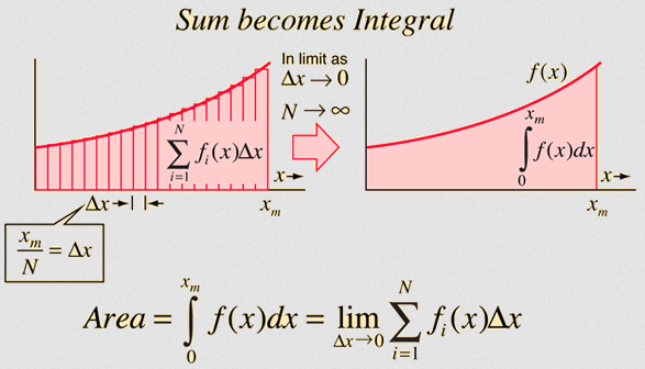
Approximation of the area of a curve using increasingly narrower rectangles. Taken from HyperPhysics

Eventually when the width of the rectanges becomes infinitesimally thin, the sum of these infinitesimally thin rectangles gives us the true area under the curve.

This technique of dividing an interval of a curve with increasingly smaller subintervals resulting in thinner and thinner rectanges to approximate area is not a mere theroetical concept but something that’s actually used in real life. I recall in one of my geography courses, the class was sent to a nearby bridge, tasked on measuring the depth of the river at different points, repeating the measurements in smaller partitions to get an approximate area of the river.

An image I found on google that looked familiar to what I learned in Geography to measure discharge. Source: Fondriest

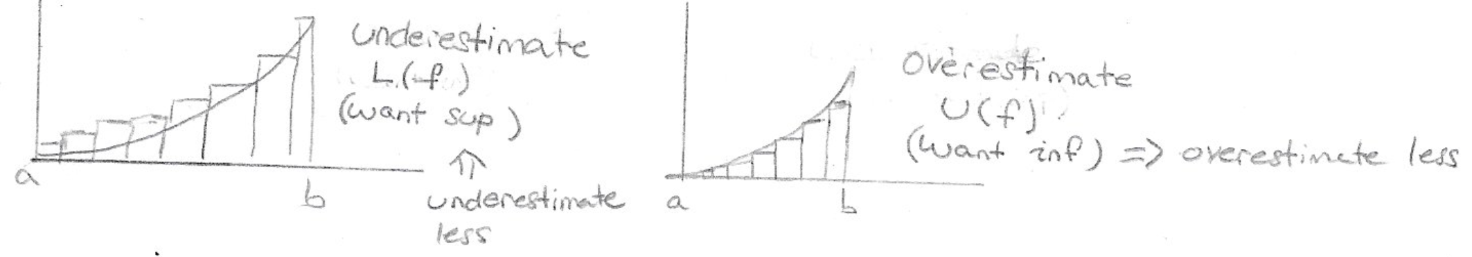
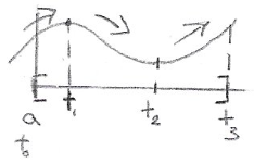
One question that may arise is how to determined the height of these rectanges as it is clear that these rectangles don’t capture the curves nicely. There are a few ways to determine the height such as grabbing the function’s value at the midpoint between each subinterval $[t_i, t_{i+1}]$, the way the author first encountered in its time as a student in computer science. But this choice can feel arbitrary with no guarantees whether the height of each subinterval under-estimates or over-estimates the true area. One elegant approach introduced in this course is to consider both cases and see if the two cases can reconcile (i.e. be equal to each other) and this approach is called Darboux Sums or Darboux Integrals.

Formally, we define a partition for a function $f$ bounded on $[a,b]$ to be:

Partition of $[a,b]$ is a finite sequence $(t_m)$ with $a = t_0 \lt t_1 \lt t_2 \lt \dots \lt t_n = b$. Thus $P = \{t_0, t_1, t_2, \dots, t_n\}$

Put simply, it is a partition is a set of ordered numbers between $a$ and $b$.

The over-estimated area is called the UPPER darboux sum and the under-estimated rectangles are called the lower darboux sum making use of the definitions of supremum and infimum encountered in the previous course. As one can easily imagine, the two darboux sums take the “max” (supremum) and “min” (infimum) of the curve within each subinterval as the height of the rectangles.

For a subset $S \subseteq [a, b]$, we let:

$M(f,S) = sup\{ f(x) : x \in S\}$ i.e. “Max height of each rectangle”

$m(f,S) = \inf\{ f(x) : x \in S \}$ i.e. “Min height of each rectange”

Thus we can formally define the upper and lower darboux sums as the following:

UPPER Darboux Sum: $U(f,P) = \sum\limits^n_{k=1} \underbrace{M(f, [t_{k-1}, t_k])}_{\text{height}} \cdot \underbrace{(t_k-t_{k-1})}_{\text{base}}$

LOWER Darboux Sum: $L(f,P) = \sum\limits^n_{k=1} \underbrace{m(f,[t_{k-1}, t_k])}_{\text{height}}\underbrace{(t_k - t_{k-1})}_{\text{base}}$

Recall the objective is to approximate and eventually get the true area under the curve by taking the sum of the area of extremely thin rectangles. Also recall that the area of a rectangle is simply width multiplied by its height.

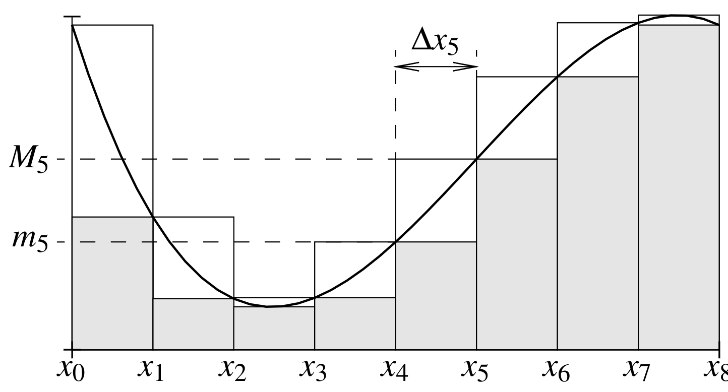
A sample of darboux sum where the lower sum is the area of the shaded rectangles and the upper sum is the area of the entire rectangles (shaded + unshaded regions). Taken from MIT OCW Real Analysis notes

One may see the upper and lower darboux sums reformulated as the following:

Upper Darboux Sum: $U(f,P) = \sum\limits^n_{k=1} M_i\Delta x_i$

Lower Darboux Sum: $L(f,P) = \sum\limits^n_{k=1} m_i \Delta x_i$

where:

$M_i = \sup\{f(x): x_{i-1} \leq x \leq x_i \}$

$m_i = \inf\{f(x): x_{i-1} \leq x \leq x_i \}$

Recall in our definition, $f$ is a bounded function on $[a,b]$ so it attains a global min and a global max value. In addition, every partition of $[a,b]$ will contain at least the endpoints $a$ and $b$. One key observation is that the local min and max are bounded by the global extremas:

• $M(f, [t_{k-1},t_k]) \leq M(f,[a,b]) = M$
• $m(f, [t_{k-1}, t_k]) \geq m(f, [a,b]) = m$

where $[t_{k-1},t_k] \subseteq [a,b]$. Intuitively, finer partitions capture the function more accurately, so the underestimate improves and the overestimate tightens (potentially decreases). Given this fact, we have the following:

$m(b-a) = m(f, [a,b])(b-a) \leq L(f,P) \leq U(f,P) \leq M(f,[a,b])(b-a) = M(b-a)$

Quick Breakdown:

\[\require{cancel} \begin{align*} U(f,P) = \sum\limits^n_{k=1} M(f,[t_{k-1},t_k])(t_k - t_{k-1}) &\leq \sum\limits^n_{k=1} M(f,[a,b])(t_k - t_{k-1})\\ &= \underbrace{M(f, [a,b])}_{\text{const}} \sum\limits^n_{k=1} (t_k-t_{k-1}) \\ &= M((\bcancel{t_1} - t_0) + (\bcancel{t_2} - \bcancel{t_1}) + \dots + (\bcancel{t_{n-1}} - \bcancel{t_{n-2}}) + (t_n - \bcancel{t_{n-1}})) \\ &= M(t_n - t_0) \\ &= M(b - a) \\ \therefore U(f,P) \leq M\sum\limits^n_{k=1} (t_k-t_{k-1}) \leq M(b-a) \end{align*}\]

Similar idea to show $m(f, [a,b])(b-a) \leq L(f,P) \leq U(f,P)$

Since $m(f,[t_{k-1},t_k]) \leq M(f, [t_{k-1}, t_k])$ (since $\inf \leq \sup$ by definition), we have $L(f,P) \leq U(f,P)$ for any single Partition P. ( Note: it is not immediately clear whether $L(f,P_1) \leq U(f.P_2)$ for different partitions $P_1,P_2$, a question we will address shortly.)

Given this proposition, we see these darboux sums are bounded and by consequence are guaranteed of the existence of an upper Darboux Integral $U(f)$ and lower Integral $L(f)$:

Upper Darboux Integral: $U(f) = \inf\{U(f,P) : P$ is a partition of $[a,b]$ $\}$. Often represented as $\overline{\int}_a^b f(x)dx$

Lower Darboux Integral: $L(f) = \sup\{L(f,P): P$ is a partition of $[a,b]$ $\}$. Often represented as $\underline{\int}_a^b f(x)dx$

Similar to how a limit exists if the LHS and RHS limits exist, we say $f$ is INTEGRABLE on $[a,b]$ if $U(f) = L(f)$ or $\overline{\int} a^b f(x)dx = \underline{\int}_a^b f(x)dx$

Darboux Integral: f is INTEGRABLE on $[a,b]$ if $U(f)=L(f)$. Often represented as $U(f)=L(f)=\int\limits_a^b f(x)dx$

where $f(x)$ can be seen as the height and $dx$ as the width of the rectangle approaching to 0.

Showing whether a function is integrable is a lot of work and thus will be omitted. Please read Ross Analysis or search online for an example. However, what I will show and find more interesting is to show a function $f$ the is NOT integrable. In Engineering, we are always given ‘‘nice” functions that always have integrals but it turns out there are functions that don’t have an “area”. One potential example is comparing the area between two functions that appear to be the same but one has finite number of holes and the other has infinitely many holes in the graph. One is integrable and the other is not.

Example:

\(f(x) = \begin{cases} 1 & x \in \mathbb{Q} \\ 0 & x \notin \mathbb{Q} \end{cases}\) on $[a,b]$. Show that f is not integrable.

Note that every interval $[t_{k-1}, t_k]$ contains a rational and irrational number (i.e. by the density of $\mathbb{Q}$)

We have: \(\begin{align*} M(f, [t_{k-1},t_k]) = 1 \forall k &\implies U(f,P)=1(b-a) = (b-a) &&\implies U(f) = b-a \\ m(f, [t_{k-1},t_k]) = 0 \forall k &\implies L(f,P)=0(b-a) = 0 &&\implies L(f) = 0 \end{align*}\)

Thus $U(f) \ne L(f)$ and by definition, $f$ is not integrable on $[a,b]$

Any engineering student should be surprised of this result, especially on the idea that one can be asked to determine if a function is integrable or not. This is one of many examples that differentiates between Math and Engineering students. Math students are expected to not take anything forgranted unless told otherwise (reality is that there are some materials that are just too complex at the moment to learn).

Previously, we saw that for any partition $P, U(f, P) \leq U(f,[a,b])$. We previously reasoned that a finer partition does a much more accurate job in capturing the function’s true behavior. Geometrically, we are summing more thinner rectangles whose lower and upper values $M_i$ and $m_i$ are tighter to the true value. Thus we can generalise the following:

Lemma 1: Let $f$ be bounded function on $[a,b]$. If $P,Q$ are partitions of $[a,b]$ with $P\subseteq Q$ (i.e. $Q$ is a “finer” partition within $[a,b]$ / has more points in the partition). Then:

$L(f,P) \leq L(f,Q) \leq U(f,Q) \leq U(f,P)$

Essentially the lemma is stating that adding points to the partition decreases the upper sum and increases the lower darboux sum. Geometrically, this would correspond to having more thinner rectangles to approximate the area more accurately.

Similarly, we can now make the claim that for any partition, the lower darboux sum will always be less than (or equal to) any upper darboux sum regardless of the partition.

Lemma 2: Let $f$ be bounded on $[a,b]$ and let $P,Q$ be partitions of $[a,b]$. Then $L(f,P) \leq U(f,Q)$

Proof: Consider the partition $P \cup Q$. Note that we know nothing about the partitions $P$ and $Q$ but we do know we can construct a larger partition $P\cup Q$ such that:

• $P\subseteq P \cup Q$
• $Q\subseteq P \cup Q$

So by the previous lemma (lemma 1),

• $L(f,P) \leq L(f, P \cup Q)$ (i.e. adding points to the partition increases the lower darboux sum)
• $U(f,P\cup Q) \leq U(f,Q)$ (i.e. adding points to the partition decreases upper darboux sum)

Chaining these two conclusion, we have: $L(f,P) \leq L(f, P \cup Q) \leq U(f,P\cup Q) \leq U(f,Q)$

Thus lemma 2 tells us tht any any lower sum is below any upper sum. But the supremum and infimum are the tightest bounds we can get. What does lemma 2 tells us about these bounds?

Lemma 3: Let $f$ be bounded on [a,b]. Then $L(f) \leq U(f)$

Previously in lemma 2, we proved that regardless of the partition, the upper darboux sum is always greater (or equal to) the lower darboux sum. This is an extension of the previous lemma but even stronger by tighting the bound such that even the GREATEST lower darboux sum is less than the LEAST upper darboux sum.

By the definition of Darboux Integrals, we know that a function is integrable if its lower and upper sum are equal (i.e. $L(f) = U(f)$). However, this definition requires us to verify this equality directly which at times can be difficult due to $U(f)$ and $L(f)$ being defined as the infima and suprema of the upper and darboux sums of an infinitely many bounded finite-partitions respectively. One can use the following characterisation to determine if a function is integrable:

Theorem 1 (Cauchy Criterion): a bounded function $f$ on $[a,b]$ is integrable $\iff \forall \epsilon > 0 \exists$ a partition $P$ of $[a,b]$ such that $U(f,P) - L(f,P) \lt \epsilon$

As one may recall from the previous course: For any $\epsilon > 0$, if the difference between two values is less than every positive $\epsilon$ then the difference must be 0.

\[\text{for any two real numbers } x, x_o, \text{ if } |x-x_o| \lt \epsilon, \forall \epsilon \gt 0 \nonumber \\ \text{then }x = x_o\]

A common example is the value $1.\overline{9} = 1.9999\dots$ (i.e. the 9 repeats infinitely many times).

No matter what $\epsilon \gt 0$ you choose, we have $2 - 1.\overline{9} \lt \epsilon$

For instance:

• $|2 - 1.9| < 0.1$
• $|2 - 1.99| < 0.01$
• $|2 - 1.999| < 0.001$

As we add more 9s, the difference gets smaller. In this limit, the difference converges to 0. Thus $2 - 1.\overline{9} = 0$ or $1.\overline{9} = 2$.

Many integration problems found in Engineering have one thing in common, they tend to be continuous? Is there a particular reason for this? It turns out that it is easy to create integration problems as long as the functions are continuous:

Theorem 2: Every continuous function $f$ on $[a,b]$ is integrable

However, sometimes a student can be blessed or cursed (depending on perspective) with a piecewise function. But in particular, these discontinuous functions tend to have one thing in common, they are montonic functions. Recall that a monotone function is a function that is either increasing or decreasing (not strictly) and do not have to be continuous. For instance, take a piecewise montonic function, the step function that jumps upward at finitely many points but never decreases. Professors don’t pose students integration problems out of nowhere, they rely on the next theorem to pose piecewise functions to students:

Theorem 3: Every monotone functions on $[a,b]$ is integrable

The next set of facts will be given without any commentary:

let $f,g$ be integrable on $[a,b]$ and let $c\in\mathbb{R}$. Then:

1. $cf$ is integrable with $\int^b_a cf = c\int^b_a f$ (scalar multiplication)
2. f+g is integrable with $\int_a^b (f + g) = \int_a^b f + \int_a^b g$ (additivity)
3. if $f(x) \leq g(x) \forall x\in [a,b]$ then $\int_a^b f(x)dx \leq \int_a^b g(x)dx$ (monotonicity)
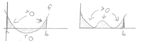
4. if $g$ is a continuous non-negative function and $\int_a^b g(x)dx = 0$ then $g(x) = 0 \forall x\in [a,b]$
5. let $a \lt c \lt b$ and if $f$ is integrable on $[a,c]$ and on $[c,b]$ then $\int_a^b f = \int_a^c + \int_c^b$ (additivity of intervals)
6. $|f|$ is integrable on $[a,b]$ and $|\int_a^b f| \leq \int_a^b |f|$ (triangle inequality)

Illustration of $\|\int_a^b f\|$ on the left and $\int_a^b \|f\|$ on the right

Previously, we stated that if $f$ is either montone or continuous, then it is integrable. But not all functions are monotone nor continuous which could severely restrict what types of curves we can compute the area under. But what if we broke the functions into separate individual pieces? That is what piecewise functions attempt to do and we shall be exploring further the integrability of such functions.

Piecewise Monotone: $f$ is called piecewise monotone on $[a,b]$ if there is a partition $P$ of $[a,b]$ such that $f$ is monotone on each open subinterval $(t_{k-1},t_k)$.

A piecewise monotone function

Piecewise Continuous: $f$ is called piecewise continuous on $[a,b]$ if there is a partition $P$ of $[a,b]$ such that $f$ is uniformly continuous on each open subinterval $(t_{k-1},t_k)$

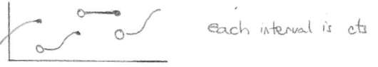
A piecewise continuous function

Theorem 4: If $f$ is piecewise continuous or (bounded) piecewise monotone on $[a,b]$, then it is integrable on $[a,b]$

With theorem 4, we have now covered the integrability of nearly all functions encountered in engineering and applied mathematics (at least at a freshman level).

Now we have covered enough to discuss the one of the biggest theorem in calculus: the fundamental theorem of calculus (FTC). Specifically we will cover the first part of FTC but essentially the fundamental theorem of calculus connects differentiation covered in the previous course with integration to show they are roughly inverses of each other. In addition, it also teaches us how to compute the integral of a function much more efficiently (at least by hand).

Theorem 5 (Fundamental Theorem of Calculus 1): if $f$ is continuous on $[a,b]$ and differentiable on $(a,b)$ and if $f’$ is integrable on $[a,b]$, then $\underbrace{\int_a^b f’(x)dx}_{\text{sum of infinitesimal changes}} = \underbrace{f(b)-f(a)}_{\text{total change}}$

The first part of the theorem tells us that integrating a derivative gives us the original function’s change. Recall that the derivative $f’(x)$ tells us the rate of change of the function $f$ at each point. Summing (i.e. integrating) all these infinitesimal changes from $a$ to $b$ should give the total change $f(b) - f(a)$.

Thus, by the fundamental theorem of calculus part 1, we have a practical method to compute definite integrals. Instead of constructing darboux sums, we can use antiderivatives.

You may see the term definite and indefinite integrals thrown around, essentially one specifies its bound and the other does not. But here’s a more complete definition:

• Definite Integral: the integral has bounds $[a,b]$ and evaluates to a single real number
• Indefinite Integral: the integral has no bounds and represents a family of antiderivatives $F(x) + C$ where $C\in\mathbb{R}$

Suppose $a \lt b$, then what would it mean if we switch the bounds around? (i.e. $\int_b^a f(x)dx$?). By the fundamental theorem of calculus part 1, we have:

\[\int_a^b f(x)dx = F(b) - F(a) \nonumber\]

So if we were to swap the bounds, we would have: $- (F(a) - F(b)) = -\int_b^a f(x)dx$

If $a \lt b$ then $\int_b^a f(x)dx = - \int_a^b f(x)dx$

If $F$ is an antiderivative of $f$ (i.e. $F’ = f$), then:

\[\int_a^b f(x)dx = F(x)|_a^b = F(b) - F(a) \nonumber\]

As a consequence, we also have the following (the second part of the FTC):

\[\frac{d}{dx}\int f(x)dx = f(x) \nonumber\]

While FTC 1 lets us compute definite integrals using antiderivatives, FTC 2 guarantees that the antiderivatives exist.

Theorem 6 (Fundamental Theorem of Calculus 2): let $f$ be integrable on $[a,b]$ and let $F(x) = \int_a^x f(t)dt$. Then $F$ is continuous on $[a,b]$. Moreover, if $f$ is continuous at $x_o\in(a,b)$ then $F$ is differentiable at $x_o$, thus $F’(x_o) = f(x_o)$.

This is a complicated way of saying the derivative undoes the integration: $\frac{d}{dx}\int f(x)dx = f(x)$

Connection to Theorem 2: Recall from Theorem 2 that every continuous function on [a,b] is integrable. By FTC 2, we not have an explicit statement that every continuous function has an antiderivative.

On the same subject, it is important to note that even if an antiderivative exists, it does NOT mean it is integrable. There is a strong reason for why the formal definition of the FTC 2 requires $f$ to be continuous (or at least integrable). Having an antiderivative is not enough.

Example:

\[F(x) = \begin{cases} x^2\sin(\frac{1}{x}) & x \neq 0 \\ \nonumber 0 & x = 0 \end{cases}\]

$F(x)$ is differentiable everywhere but DIFFERENTIABILITY $\bcancel{\implies}$ Integrability

For $x \neq 0, f(x) = F’(x) = 2x\sin(\frac{1}{x}) + x^2(\cos(\frac{1}{x}))(\frac{-1}{x^2}) = 2x\sin(\frac{1}{x}) - \cos(\frac{1}{x})$

As $x\to 0$, it widly oscillates between 1 and -1 according to Wikipedia and thus is discontinuous around the neighborhood $x = 0$. With some math I won’t get into, this function apparently broke the accepted knowledge of what functions were differentiable everywhere and its derivative was bounded, the derivative was always integrable. As this is a first-year course in Calculus, we are strictly referring Integrability as Riemann/Darboux integrable. Using the definitions presented in the blog, this function is not Darboux Integrable.

---

Integration Techniques

Thus far we have covered what it means to take an integral of a function and what sorts of functions are integrable. Let us now use the fundamental theorem of calculus part 1 and various integration techniques to compute integrals.

Here are some basic integration rules to know:

• constant: $\int a dx = ax + C, a\in\mathbb{R}$
• power rule: $\int x^n dx = \frac{x^{n+1}}{n+1} + C, n\neq -1$
• reciprocal: $\int \frac{1}{x}dx = \ln |x| + C$
• sum/difference: $\int [f(x) \pm g(x)]dx = \int f(x)dx \pm \int g(x)dx$

Exponential and Logarithmic Functions:

• $\int e^x dx = e^x + C$
• $\int a^x dx = \frac{a^x}{\ln(a)} + C, a \gt 0, a\neq 1$
• $\int \ln(x) dx = x\ln(x) - x + C$
• $\int \frac{1}{x\ln (x)} dx = \ln |\ln(x)| + C$

Trigonometric Functions:

• $\int \cos(x) dx = \sin(x) + C$
• $\int \sin(x) dx = -\cos(x) + C$
• $\int \sec^2(x)dx = \tan(x)+C$
• $\int \sec(x)\tan(x)dx = \sec(x) + C$
• And many more …

The issue with computing integrals is that it tends to be an exercise of memorisation and practice to know what techniques to use and what the anti-derivatives are. Hence why I don’t find this section particular interesting. But nonethless, it is important to go through different common integration techniques one needs to know to survive their calculus course.

Most functions have no anti-derivatives, and thus Mathematicians have discovered or invented techniques to tackle each problem. Before the release of LLMs, integration calculators were notorious for giving complicated solutions to integral problems as they often employed their own common generic integration techniques to solve the problem which weren’t student friendly solutions.

The most basic and fundamental integration technique is substitution which is essential to understand. It is the most fundamental integration technique that gets employed in many other integration techniques so it is primordial to master it.

Substitution Rule: $\int_a^b f(g(x))g’(x)dx = \int_{u(a)}^{u(b)} f(u)du, $ where $u = g(x)$

The substitution rule works by recognising composite functions. When you see an integrand with “chain rule” structure, you can often times simplify by substituting the problem to an easier integral. This looks more daunting than it should be so let’s look at a simple example:

Example: $\int_0^1 e^{2x} dx$

The integrand $e^{2x}$ is composite: $f(x) = e^x$ and $g(x)$ = 2x, so $f(g(x)) = e^{2x}$.

Our basic rule $\int e^x dx = e^x + C$ does not directly apply because of the coefficient 2 on $x$. This is where substitution helps:

Let $u = 2x$. Then:

\[\begin{align*} u = 2x, \qquad \frac{du}{dx} &= 2\\ dx &= \frac{du}{2} \end{align*}\]

Thus we can rewrite the integral as:

\[\begin{align*} \int e^{2x} dx = \int e^u \frac{du}{2} = \frac{1}{2}\int e^u du \end{align*}\]

The integrand now is in the correct form and thus is solvable.

\[\begin{align*} \frac{1}{2}\int e^u du = \frac{1}{2} e^u + C \end{align*}\]

However, as the question posed a definite integral, we must account for the bounds? There are two approaches:

1. Change of Bounds Determine what the lower and upper bounds are by computing $u(a)$ and $u(b)$ are

   \[x = 0: u(0) = 2(0) = 0 \\ \nonumber x = 1: u(1) = 2(1) = 2 \nonumber\]

   So now we can integrate directly:

   \[\begin{align*} \frac{1}{2}\int_0^2 e^u du &= \frac{1}{2} e^u|_0^2 \\ &= \frac{1}{2}[e^2 - e^0] \\ &= \frac{e^2 - 1}{2} \end{align*}\]

   The benefit with this approach is that we can work entirely in terms of $u$, there is no need to substitute back

2. Substitute Back: Solve the indefinite integral first, then substitute back $u = 2x$ before evaluating bounds:

   \[\begin{align*} \int_0^1 e^{2x}dx &= \frac{1}{2}\int_{x=0}^{x=1} e^u du\\ &= \frac{1}{2} e^u|_{x=0}^{x=1} \\ \end{align*}\]

   As the bounds are respect to $x$, let’s substitute back our original function $u = 2x$

   \[\begin{align*} \frac{1}{2} e^u|_{x=0}^{x=1} &= \frac{1}{2}e^{2x}|_0^1 \\ &= \frac{1}{2}[e^{2(1)} - e^{2(0)}] \\ &= \frac{e^2 - e^0}{2} \\ &= \frac{e^2 - 1}{2} \end{align*}\]

I always stress to my students to verify their work if feasible (i.e. if time permits and isn’t overly complex to do so) by taking the derivative of their indefinite integral and see if it matches the original integrand:

\[\begin{align*} (\frac{e^u}{2} + C)' &= \left(\frac{e^u}{2}\right)(u') \\ &= (\frac{e^{2x}}{2})(2x)' \\ &= (\frac{e^{2x}}{\bcancel{2}})(\bcancel{2}) \\ &= \boxed{e^{2x}} \end{align*}\]

This matches our original integrand $e^{2x}$, so we can be confident our integration is correct.

This verification step catches algebraic errors, wrong coefficients, and misapplied rules. If your derivative doesn’t match the integrand, you have made a mistake somewhere.

The Substitution rule has various names including u-subitution rule or change of variables but the most important thing to take from this rule is its ability to simplify the integrand and it can potentially achieve this by cancelling a term due to the derivative of $u$.

Example:

For instance, consider the following problem: $\int \frac{x}{x^2+1}dx$

This problem looks very complicated but if we let $u = x^2+1$ then:

\[\begin{align*} u = x^2+1 \implies \frac{du}{dx} &= 2x\\ \frac{du}{2x} &= dx \end{align*}\]

Resulting in the following:

\[\begin{align*} \int \frac{x}{x^2+1}dx &= \int \frac{\bcancel{x}}{u}\left(\frac{du}{2\bcancel{x}}\right)\\ &= \frac{1}{2} \int \frac{1}{u}du \\ &= \frac{1}{2} \ln(u) \\ &= \boxed{\frac{1}{2} \ln(x^2+1)} \end{align*}\]

Check:

\[\begin{align*} \frac{1}{2} (\ln(x^2+1) &= \frac{1}{2} \frac{1}{x^2+1} (x^2+1)') \\ &= \frac{1}{\bcancel{2}} \left(\frac{1}{x^2+1}\right)(\bcancel{2}x) \\ &= \boxed{\frac{x}{x^2+1}} \end{align*}\]

The next integration technique is called Integration By Parts, useful when the integrand is a product of two separate functions where one becomes simpler when differentiated:

Integration By Parts: $\int uv’dx = uv - \int vdu$

Example: $\int x\sin(x) dx$

The integrand is a product of two functions $x$ and $\sin(x)$.

Choosing which function is to be $u$ or $v’$ takes practice but in general, I like to always default choosing $u$ to be a polynomial function like the linear function $x$ if applicable, else consider whose integral (antiderivative) is the least difficult. According to Wikipedia, there is the LIATE rule, a rule I never heard of till now. This rule is a general guide to choosing the $u$:

1. L Logarithmic functions
2. I Inverse Trigonometric Functions: $\arctan(x), \text{arcsec}(x)$, etc.
3. A algebraic functions such as polynomials
4. T: trigonmetric functions: $\sin(x), \tan(x)$, etc.
5. E: Exponential functions

Based on my personal experience and this rule, choose $u = x$ and $v’ = \sin(x)$. Thus we have:

\[\begin{align*} u &= x \qquad v' = \sin(x) \\ \frac{du}{dx} &= 1 \qquad v \ = -\cos(x) \end{align*}\]

Apply the integration by parts rule, we have:

\[\begin{align*} \int x\sin(x) dx &= uv - \int vdu\\ &= -x\cos(x) - \int -\cos(x)dx \\ &= -x\cos(x) + \int \cos(x)dx \\ &= \boxed{-x\cos(x) + \sin(x) + C} \end{align*}\]

Check: \(\begin{align*} (-x\cos(x) + \sin(x) + C)' &= \bcancel{-\cos(x)} + (\bcancel{-}x)(\bcancel{-}\sin(x)) + \bcancel{\cos(x)} + 0 \\ &= \boxed{x\sin(x)} \end{align*}\)

One trick to recall the rule is to start with the product rule and get the left side to be in the form $uv’$:

\[\begin{align*} (uv)' &= u'v + v'u \\ uv' &= (uv)' - u'v \\ \int uv' &= \int (uv)' - \int u'v \\ \int uv' &= \boxed{uv - \int v du} \end{align*}\]

From my time as a teaching assistant in Calculus for Engineers, I learned there is an integration by parts table that one could adopt to organise the various substitution required to the problem. This is particular useful when the question requires to apply the rule multiple times. Perhaps I’ll cover this in the future.

The integration by parts can be an effective tool to solve problems that doesn’t seem to be a product of two functions such as $\int \ln(x)dx$. Recall that a product between 1 and any function is the function itself. This itself is a product:

Example:

\[\begin{align*} \int \ln(x) &= \int \ln(x) \cdot 1 \\ \end{align*}\]

Based on LIATE rule, logarithmic takes precedent over algebraic functions thus take $u = \ln(x)$

\[\begin{align*} u &= \ln(x) & dv &= 1dx \\ \frac{du}{dx} &= \frac{1}{x} \implies \boxed{du = \frac{1}{x}dx} & v &= x \end{align*}\]

Thus,

\[\begin{align*} \int \ln(x)dx &= x\ln(x) - \int \bcancel{x}(\frac{dx}{\bcancel{x}} \\ &= x\ln(x) - \int dx \\ &= \boxed{x\ln(x) - x + C} \end{align*}\]

Check:

\[\begin{align*} (x\ln(x) - x + C)' &= \ln(x) + \bcancel{x}\left(\frac{1}{\bcancel{x}}\right) - 1 + 0 \\ &= \ln(x) + 1 - 1 \\ &= \boxed{\ln(x)} \end{align*}\]

Trigonometric Substitution:

Consider the following integration: $\int \frac{1}{\sqrt{4-x^2}}dx$. One’s first instinct may be to utilise substitution or integration by parts. However this will likely end poorly. It turns out this class of problems requires trigonometric substitution. Whenever one sees the following expressions in the following form, it is best to consider trigonmetric substitution first:

• $\sqrt{a^2-x^2}$
• $\sqrt{a^2+x^2}$
• $\sqrt{x^2-a^2}$

The key to knowing what trig to substitute x for lies in the identities which are convienently layed out below:

Trigonometric Substitution:

form	substitution	identity used
$\sqrt{a^2-x^2}$	$x=a\sin\theta$	$1-\sin^2\theta = \cos^2\theta$
$\sqrt{a^2+x^2}$	$x=a\tan\theta$	$1+\tan^2\theta = \sec^2\theta$
$\sqrt{x^2-a^2}$	$x=a\sec\theta$	$\sec^2\theta-1=\tan^2\theta$

Let’s see how this works in practice by looking at the motivating example: $\int\frac{1}{\sqrt{4-x^2}}dx$

Step 1: Identify the form and choose a substitution

The expression $\sqrt{4-x^2}$ fits the form $\sqrt{a^2-x^2}$ where $a = 2$.

By the table above, use $x = 2\sin\theta$

Step 2: Compute the derivative and simplify the square root

From $x = 2\sin\theta$: \(\begin{align*} x &= 2\sin\theta \\ \frac{dx}{d\theta} &= 2\cos\theta \\ dx &= \boxed{2\cos\theta d\theta} \end{align*}\)

Simplify $\sqrt{4-x^2}$:

\[\begin{align*} \sqrt{2^2-x^2} &= \sqrt{2^2 - (2\sin\theta)^2} \\ &= \sqrt{4 - 4\sin\theta^2} \\ &= \sqrt{4(1 - \sin\theta^2)} \\ &= \sqrt{4}\sqrt{1 - \sin\theta^2} \\ &= 2\sqrt{\cos^2\theta} \\ &= 2|\cos\theta| \end{align*}\]

Let’s restrict $\theta \in [\frac{-\pi}{2},\frac{\pi}{2}]$ so $\cos\theta \geq 0$. Thus $|\cos\theta| = \cos\theta$.

Step 3: Substitute into the integral

\[\begin{align*} \int\frac{1}{\sqrt{4-x^2}}dx &= \int\frac{1}{2\cos\theta}dx \\ &= \int \frac{1}{\bcancel{2\cos\theta}} (\bcancel{2\cos\theta} d\theta) \\ &= \int d\theta \\ &= \theta + C \end{align*}\]

Step 4: Substitute $x$ back

Recall that $x = 2\sin\theta$,

\[\begin{align*} x &= 2\sin\theta \\ \frac{x}{2} &= \sin\theta \\ \theta &= \arcsin(\frac{x}{2}) + C \end{align*}\]

Thus, $\int\frac{1}{\sqrt{1-x^2}}dx = \theta = \arcsin(\frac{x}{2})$

Check:

\[\begin{align*} (\arcsin(\frac{x}{2}))' &= \frac{1}{\sqrt{1-(\frac{x}{2})^2}}\left(\frac{x}{2}\right)' \\ &= \frac{1}{\sqrt{1-\frac{x^2}{4}}}\left(\frac{1}{2}\right) \\ &= \frac{1}{2\sqrt{1-\frac{x^2}{4}}} \\ &= \frac{1}{\sqrt{4}\sqrt{1-\frac{x^2}{4}}} \\ &= \frac{1}{\sqrt{4(1-\frac{x^2}{4}})} \\ &= \boxed{\frac{1}{\sqrt{4-x^2}}} \end{align*}\]

Hopefully, this motivating example gave you a glimpse of the power of trig substitution. There are many more interesting questions that one could solve that requires one to recall special triangles and the SOH CAH TOA rule to convert trig functions in respect to $\theta$ back to $x$ but will be a story for another time. But as an exercise, derive the area of a circle of radius r, you should get $\pi r^2$.

Partial Fractions:

Another class of rational functions that can be integrated utilises a technique called partial fractions but this only works (from my memory) with rational functions whose numerator and denominators are polynomials. The reason is quite simple, this technique relies on decomposing rational functions into smaller pieces.

Decomposition: for a rational function $\frac{p(x)}{q(x)}, it can always be decomposed into smaller pieces, each of which can be integrated

Example: $\frac{1}{x^2-1} = \frac{\frac{1}{2}}{x-1} - \frac{\frac{1}{2}}{x+1}$

A condition for partial fractions in general is that deg$(p(x)) \lt $deg$q(x)$. If deg$(p(x)) \geq $deg$q(x)$, use polynomimal long divisionto separate the polynomial part from the remainer:

\[\frac{p(x)}{q(x)} = Q(x) + \frac{r(x)}{q(x)}\nonumber\]

Then apply partial fractions to $\frac{r(x)}{q(x)}$, where now deg$(r) \lt $deg$(q)$.

The form of the partial fraction decomposition depends on the type of factors in the denominator:

• Case 1: Distinct Linear Factors

  After factoring, if the denominators have distinct roots then we have each term in the form: $\frac{A}{ax+b}$

• Case 2: Repeated Linear Roots

  After factoring, if the denominator has repeated roots (i.e. $(ax+b)^n$), then we need to create a term for each and every power up to $n$:

  \[\begin{align*} \frac{A_1}{ax+b} + \frac{A_2}{(ax+b)^2} + \frac{A_3}{(ax+b)^3} + \cdots + \frac{A_n}{(ax+b)^n} \end{align*}\]

• Case 3: Distinct Irreducible Quadratic Factors

  Not all quadratics are reducible using real numbers and thus remain in the form: $ax^2+bx+c$. Then the term will have a corresponding partial fraction term: $\frac{Ax+B}{ax^2+bx+c}$

• Case 4: Repeated Quadratic Factors

  Similar to case 2, if you notice irredicuble quadratic terms in the denominator of our rational functions, we need to build up the terms repeatedly with higher powers:

  \[\begin{align*} \frac{A_1x+B_1}{ax^2+bx+c} + \frac{A_2x+B_2}{(ax^2+bx+c)^2} + \frac{A_3x+B_3}{(ax^2+bx+c)^3} + \cdots + \frac{A_nx+B_n}{(ax^2+bx+c)^n} \end{align*}\]

The constant terms $A_i, B_i$ are determine using linear algebra. Let’s go through a simple example:

$\int \frac{1}{4x^2-1}dx$

Immediately you should notice that this is in the form $a^2-b^2$ thus we can utilise what we saw in Highschool (differences in squares): $a^2-b^2 = (a+b)(a-b)$: $4x^2-1 = 4x^2 - 1^2 = (2x+1)(2x-1)$

Based on our general rule, we have two distinct roots and thus each term corresponds to a linear root: $\frac{A}{ax+b}$. Thus we reduced the rational function into the following parts:

\[\begin{align*} \int \frac{1}{4x^2-1}dx &= \int \frac{1}{(2x+1)(2x-1)} \\ &= \int \frac{A}{2x+1} dx + \int \frac{B}{2x-1}dx \\ &= \int \frac{A(2x-1) + B(2x+1)}{(2x+1)(2x-1)} \\ &= \int \frac{2x(A+B) + (B-A)}{(2x+1)(2x-1)} \end{align*}\]

From here, we are left with two unknowns: $A, B$:

The idea is to group each order as its own term such that we can solve the coefficients since the functions ${1, x, x^2, x^3, \dots}$ are linearly independent in the vectorspace for $x\in\mathbb{R}$

\[\begin{align*} 1 &= 2x(A+B) + (B-A) \\ 0x + 1 &= 2x(A+B) + (B-A) \end{align*}\]

Thus we have:

• 1: $1 = B-A \implies B = 1 + A$

• $x$: $0 = A+B$

  \[\begin{align*} 0 &= A+B\\ A &= -B \\ &= -(1+A) \\ A &= -1 -A \\ 2A &= -1 \\ A &= \boxed{\frac{-1}{2}} \end{align*}\]

Plugging $\boxed{A = \frac{-1}{2}}$ into $B = 1 + A$, we have $\boxed{B = \frac{1}{2}}$

Or alternatively, we could try to utilise nice numbers such as 0 or the roots to the equation to cancel out some terms to retrieve $A$ and $B$ more quickly:

Consider: $1 = A(2x-1) + B(2x+1)$

• if $x = \frac{1}{2}$: \(\begin{align*} 1 &= A(0) + B(2) B &= \frac{1}{2} \end{align*}\)
• if $x = \frac{-1}{2}$: \(\begin{align*} 1 &= A(-2) + B(0) A &= \frac{-1}{2} \end{align*}\)

By choosing the roots, we remove one term at a time, isolating each constant. This is faster than expanding and comparing coefficients. Plugging in nice numbers such as $x = 0$ at times is sufficient as well.

Therefore, the integral is now:

\[\begin{align*} \int \frac{1}{4x^2-1}dx &= \frac{-1}{2} \int \frac{1}{(2x+1)} dx + \frac{1}{2}\int \frac{1}{2x-1}dx \end{align*}\]

A much more manageable smaller pieces of integrals that can now be solved:

\[\begin{align*} \int \frac{1}{4x^2-1}dx &= \frac{-1}{2} \int \frac{1}{(2x+1)} dx + \frac{1}{2}\int \frac{1}{2x-1}dx \\ &= \left(\frac{-1}{2}\right)\left(\frac{1}{2}\right)\ln|2x+1| + \frac{1}{2}\left(\frac{1}{2}\right) \ln|2x-1| \\ &= \frac{1}{4}\ln|2x-1| - \frac{1}{4}\ln|2x+1| \\ &= \boxed{\frac{1}{4}\ln\left|\frac{2x-1}{2x+1}\right| + C} \end{align*}\]

Check:

\[\begin{align*} \left(\frac{1}{4}\ln|2x-1| - \frac{1}{4}\ln|2x+1|\right) + C &= \left(\frac{1}{4}\right)\left(\frac{1}{2x-1}\right)(2x-1)' - \left(\frac{1}{4}\right)\left(\frac{1}{2x+1}\right)(2x+1)' \\ &= \frac{1}{2}\left[\frac{1}{2x-1} - \frac{1}{2x+1}\right] \\ &= \frac{1}{2}\left[\frac{2x+1 - (2x-1)}{(2x+1)(2x-1)}\right] \\ &= \frac{1}{2}\left[\frac{2x + 1 - 2x + 1}{(2x+1)(2x-1)}\right] \\ &= \frac{1}{\bcancel{2}}\left[\frac{\bcancel{2}}{4x^2-1}\right] \\ &= \boxed{\frac{1}{4x^2 - 1}} \end{align*}\]

Improper Integrals:

Thus far, we have studied integral of functions over closed, bounded intervals $[a,b]$. Even our integrability conditions required bounded domains. But there is another class of integrals called the IMPROPER INTEGRALS, where either:

• the domain extends to infinity OR
• the function has a discontinuity at an end point

\[\int_1^\infty \frac{1}{x^2}dx \nonumber\]

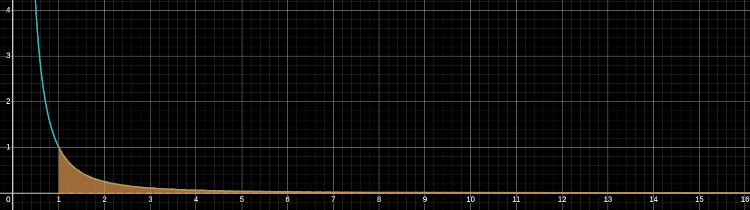
The area under the curve of $\frac{1}{x^2}$ from $x\geq 1$

The remarkable result is that even though the domain is unbounded, the area is finite (equals to 1).

Improper Integrals: Without loss of generality, consider $[a, b)$, where $b$ is finite or $\infty$. Let $f$ be defined on $[a,b)$ and integrable on each $[a,d]$ for $a \lt d \lt b$.

We define $\int_a^b f(x)dx = \lim\limits_{d\to b^{-}}\int_a^d f(x)dx$, provided the limit exists

Consider the example: $\int_1^\infty \frac{1}{x^2}dx$:

\[\begin{align*} \int_1^\infty \frac{1}{x^2}dx &= \lim\limits_{d\to\infty} \int_1^d \frac{1}{x^2}dx \\ &= \lim\limits_{d\to\infty} \left(\frac{x^{-1}}{-1}\bigg|_1^d\right) \\ &= \lim\limits_{d\to\infty} \left( \frac{-1}{d} - \left(-\frac{1}{1}\right) \right) \\ &= \lim\limits_{d\to\infty} \left(1 + \frac{-1}{d}\right) \\ &= 1 \end{align*}\]

Let’s consider the region between $(0, 1]$. Intuitively, since the interval length is only 1 compared to $[1, \infty)$ which has infinite length, surely the area should be finite, right?

Wrong! It turns out that $\int_0^1 \frac{1}{x^2}dx$ diverges (or converges to $\infty$), despite the bounded domain.

As $0\notin dom(f)$, the integral is improper:

\[\begin{align*} \int_0^1 \frac{1}{x^2} &= \lim\limits_{d\to 0^+} \int_d^1 \frac{1}{x^2}dx \\ &= \lim\limits_{d\to 0^+} \left(\frac{x^{-1}}{-1}\bigg|_d^1\right) \\ &= \lim\limits_{d\to 0^+} \left( \frac{-1}{1} - \left(-\frac{1}{d}\right) \right) \\ &= \lim\limits_{d\to 0^+} \left(\frac{1}{d} - 1\right) \\ &= \infty \end{align*}\]

We can generalise this behavior by solving $\int_1^\infty \frac{1}{x^p}$ and $\int_0^1 \frac{1}{x^p}$.

\[\begin{align*} \int_0^1 = \begin{cases} \infty & p \geq 1 \\ \frac{1}{1-p} & p \lt 1 \end{cases} \end{align*}\]

and

\[\begin{align*} \int_1^\infty = \begin{cases} \frac{1}{p-1} & p \gt 1 \\ \infty & p \leq 1 \end{cases} \end{align*}\]

Integral	p < 1	p = 1	p > 1
$\int_0^1 \frac{1}{x^p} dx$	Converges	Diverges	Diverges
$\int_1^\infty \frac{1}{x^p}dx$	Diverges	Diverges	Converges

What we can conclude from the past few examples is that the size of the domain does not matter, but rather its the behaviour of the function within the interval that matters. An obvious result but sometimes taken forgranted.

Recall in the previous course, we explore the $p$-test which stated:

P-Series: $\sum \frac{1}{n^p}$ converges if $p \gt 1$ and diverges if $p\leq 1$

$\int_1^\infty \frac{1}{x^p}dx$ and $\sum\limits_{n=1}^\infty \frac{1}{n^p}$ both diverge when $p \leq 1$. Is there a pattern between the two? Turns out yes and it’s called the integral test:

Integral Test for Infinite Series: let $N\in\mathbb{Z}$ and suppose $f(x)$ is continuous, decreasing and non-negative on $[N, \infty]$ then $\sum\limits_{n=N}^\infty f(n)$ converges/diverges $\iff$ $\int_N^\infty f(x)dx$ converges/diverges respectively

It can be difficult to determine whether an infinite series converge or diverge, so the Integral test will be a handy tool.

If an integral is improper at both endpoints, one must split it up into 2 separate improper integrals and evaluate each integral separately.

Improper Integrals (Improper at Both Ends): If $\int_a^b f(x)dx$ is improper at both ends, then by definition $\int_a^b f(x)dx = \int_a^c f(x)dx + \int_c^b f(x) dx$, where $c\in(a,b)$ and $f$ is defined at $c$.

If one of the two improper integrals evaluates to $\infty$ and the other is $-\infty$, then the integral is undefined

For instance, consider the following example:

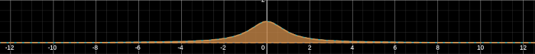
Area of $\frac{1}{1+x^2}$

\[\begin{align*} \int_{-\infty}^\infty \frac{1}{x^2+1}dx \end{align*}\]

The two endpoints are improper and thus are broken into two pieces:

1. $\int_{-\infty}^0 \frac{1}{x^2+1}dx$
2. $\int_0^\infty \frac{1}{x^2+1}dx$

Important: Both pieces must converge for the original integral to converge. If even one diverges, the entire integral diverges.

The problem will be left as an exercise to the readers.

A common mistake is to compute an improper integral that is improper at both endpoints as one:

\[\begin{align*} \int_{-\infty}^\infty x dx &= \lim\limits_{d\to\infty}\int_{-d}^d xdx \\ &= \lim\limits_{d\to\infty} \left(\frac{x^2}{2}\bigg|_{-d}^d\right) \\ &= \lim\limits_{d\to\infty} \frac{d^2}{2} - \left(\frac{(-d)^2}{2}\right) \\ &= 0 \quad\text{ THIS IS WRONG} \end{align*}\]

By symmetry, this seems fine. But it is invalid because the integral is improper at both endpoints and thus must be split. We will soon see that the integral is in fact undefined:

Left Piece:

\[\begin{align*} \int_{-\infty}^0 x dx &= \lim\limits_{d\to\infty}\int_{-d}^0 xdx \\ &= \lim\limits_{d\to\infty} \frac{x^2}{2}\bigg|_{-d}^0 \\ &= \lim\limits_{d\to\infty} \left(\frac{0^2}{2} - \frac{(-d)^2}{2}\right) \\ &= 0 - \infty \\ &= -\infty \end{align*}\]

Right Piece:

\[\begin{align*} \int_{0}^\infty x dx &= \lim\limits_{d\to\infty}\int_{0}^\infty xdx \\ &= \lim\limits_{d\to\infty} \frac{x^2}{2}\bigg|_0^\infty \\ &= \lim\limits_{d\to\infty} \left(\frac{d^2}{2} - \frac{0^2}{2}\right) \\ &= \infty \\ \end{align*}\]

As one diverges to $-\infty$ while the other to $\infty$, we cannot treat the two as equal opposites and thus they do not cancel each other.

---

Power Series

Have you ever wondered how a calculator computes transcendentals such as $\sin x$ or $e^x$? The secret lies in power series, infinite sums of terms that represent these functions accurately. Think of a power series as a polynomial with infinitely many terms. For instance, consider $e^x$, it can be represented as the following:

\[\begin{align*} e^x = 1 + x + \frac{x^2}{2} + \frac{x^3}{6} + \frac{x^4}{24} + \cdots = \sum\limits_{n=0}^\infty \frac{x^n}{n!} \end{align*}\]

Evidentally, calculators must give an answer and thus cannot sum an infinite amount of terms. Therefore, it is important for us to know how many terms are enough to sufficiently give us an answer that is precise to our needs. This approximation is a subject that is also explored in this course.

Power Series: let $(a_n)_{n=0}^\infty$ be a sequence. The series $\sum\limits_{n=0}^\infty a_n x^n$ is called a power series (centered at 0) with coefficients $(a_n)^\infty_{n=0}$

In the previous course, we studied series convergence:

\[\sum_{n=0}^{\infty} a_n \nonumber\]

And utilised tests (p-test, ratio test, comparison test, etc.) to answer whether the series converge or diverge. With power series, we face a new question:

\[\sum_{n=0}^{\infty} a_n x^n \nonumber\]

For which values of $x$ does this series converge? The questions and answers we seek is no longer simply whether a series converge but also to determine the interval of x-values where converge occurs (called the radius of convergence). In power series, convergence is dependent on $x$, for instance:

\[\begin{align*} \sum\limits_{n=0}^\infty n^n x^n \end{align*}\]

By ratio test:

\[\begin{align*} \lim\limits_{n\to\infty} |n^n x^n|^\frac{1}{n} = \lim_{n \to \infty} n|x| = \begin{cases} \infty & x \neq 0 \\ 0 & x = 0 \end{cases} \end{align*}\]

This power series converges only when $x = 0$. This is consistent to a fact about power series, they always converge when $x = 0$ unsurprisingly.

Fact 1: every power series coverges at $x = 0$ as $0^0 = 1$

Consider another example: $\sum\limits_{n=0}^\infty x^n$. By geometric series where $x = r$, we have $\sum\limits_{n=0}^\infty x^n = \frac{1}{1-x}$ which converges when $|x| \lt 1$.

Thus, in this example, we have the power series converge when $x \lt 1$, a larger interval compare to the previous example which converged only at one point.

Now consider the last example: $e^x = \sum\limits_{n=0}^\infty \frac{x^n}{n!}$. This is a power series with $a_n = \frac{1}{n!}$. By fixing $x$ and applying the ratio test, we have the following:

\[\begin{align*} \lim\limits_{n\to\infty} \bigg|\frac{\frac{1}{(n+1)!} x^{n+1}}{\frac{1}{n!} x^n}\bigg| &= \lim\limits_{n\to\infty} \bigg| \bcancel{\left(\frac{n!x^n}{n!x^n}\right)} \frac{x}{(n+1)}\bigg|\\ &= \lim\limits_{n\to\infty} \frac{|x|}{n+1} \\ &= |x| \lim\limits_{n\to\infty} \frac{1}{n+1} \\ &= 0 \lt 1 \end{align*}\]

So by ratio test, $\sum\limits_{n=0}^\infty \frac{x^n}{n!}$ converges and since $x$ was arbitrary, it converges $\forall x\in\mathbb{R}$

The last 3 examples illustrates 3 possibilities for a power series $\sum a_nx^n$, it can either:

1. converge only at $x = 0 \implies R = 0$
2. converges for all $x$ in a bounded interval certered at 0
3. converges $\forall x\in\mathbb{R} \implies R = \infty$

Theorem 7 (Radius of Convergence): For the power series $\sum\limits_{n=0}^\infty a_n x^n$, let $R = \lim\limits_{n\to\infty} \bigg| \frac{a_n}{a_{n+1}} \bigg|$

Then $\sum\limits_{n=0}^\infty a_n x^n$ converges absoutely for $|x| \lt R$ and diverges for $|x| \gt R$

where $R$ is called the radius of convergence of $\sum\limits_{n=0}^\infty a_n x^n$

Note: Endpoints to be checked separately

Example: Find radius of convergence of $\sum\limits_{n=1}^\infty \frac{x^n}{n}$

$\sum\limits_{n=1}^\infty \frac{x^n}{n} = \sum\limits_{n=1}^\infty a_nx^n$, where $a_n=\frac{1}{n}$

\[\lim\limits_{n\to\infty} \bigg|\frac{a_n}{a_{n+1}}\bigg| = \lim\limits_{n\to\infty} \bigg|\frac{\frac{1}{n}}{\frac{1}{n+1}}\bigg| = \lim\limits_{n\to\infty} \bigg|\frac{n+1}{n}\bigg| = 1 \nonumber\]

Since this limit exists, $R = 1$. Hence, $\sum\limits_{n=1}^\infty \frac{x^n}{n}$ converges $\forall x$ with $|x| \lt 1$ i.e. $\forall x\in(-1,1)$

We need to check the endpoints separately since it may converge over there as well.

For $x = -1$:

\[\sum\limits_{n=1}^\infty \frac{x^n}{n} = \sum\limits_{n=1}^\infty \frac{(-1)^n}{n}\nonumber\]

This converges by the alternating series test.

For $x = 1$:

\[\sum\limits_{n=1}^\infty \frac{x^n}{n} = \sum\limits_{n=1}^\infty \frac{1^n}{n}\nonumber\]

Recall this is a harmonic series and thus diverges

Thus, $\sum\limits_{n=1}^\infty \frac{x^n}{n}$ converges for $x\in[1, 1)$.

Note that the radius of convergence is still 1, but we call $[-1,1)$ the interval of convergence which could be larger than your radius of convergence itself.

Center of Power Series: Power series can be centered at values other than 0. For a power series centered at $x = x_o$, it is represented as $\sum\limits_{n=0}^\infty a_n(x-x_o)^n$

The power series converges on $|x-x_o|\lt R$ and diverges on $|x-x_o| \gt R$. Again, the endpoints needs to be checked separately.

Example: Find the interval of convergence of $\sum\limits_{n=0}^\infty \frac{5^n}{n}(x-2)^n$

1. Find the radius of convergence: $a_n = \frac{5^n}{n}$ so:

   \[\begin{align*} \lim\limits_{n\to\infty} \bigg|\frac{a_n}{a_{n+1}}\bigg| &= \lim\limits_{n\to\infty}\bigg|\frac{\frac{5^n}{n}}{\frac{5^{n+1}}{n+1}} \\ &= \lim\limits_{n\to\infty} \left( \frac{5^n}{n} \right)\left(\frac{n+1}{5^{n+1}}\right) \\ &= \frac{1}{5}\lim\limits_{n\to\infty} \frac{n+1}{n} \\ &= \frac{1}{5} \end{align*}\]

   Thus $\boxed{R = \frac{1}{5}}$ and $x\in(x_o - R, x_o + R) = (2 - \frac{1}{5}, 2 + \frac{1}{5}) = (\frac{9}{5}, \frac{11}{5})$

2. Check endpoints: For $x = \frac{9}{5}$:

   \[\begin{align*} \sum\limits_{n=1}^\infty\frac{5^n}{n}\left(\frac{9}{5} - 2\right)^n &= \sum\limits_{n=1}^\infty\frac{5^n}{n}\left(\frac{-1}{5}\right)^n \\ &= \sum\limits_{n=1}^\infty\frac{5^n}{n}\left(\frac{(-1)^n}{5^n}\right) \\ &= \sum\limits_{n=1}^\infty\frac{\bcancel{5^n}}{n}\left(\frac{(-1)^n}{\bcancel{5^n}}\right) \\ &= \sum\limits_{n=1}^\infty \frac{(-1)^n)}{n} \end{align*}\]

   By the alternating test, the series converges

   For $x = \frac{11}{5}$:

   \[\begin{align*} \sum\limits_{n=1}^\infty\frac{5^n}{n}\left(\frac{11}{5} - 2\right)^n &= \sum\limits_{n=1}^\infty\frac{5^n}{n}\left(\frac{1}{5} - 2\right)^n \\ &= \sum\limits_{n=1}^\infty \frac{1}{n} \end{align*}\]

   As this is a harmonic series, the series converges at $x= \frac{11}{5}$

Therefore, the interval of convergence for this power series centered at $x_o = 2$ is $[\frac{9}{5}, \frac{11}{5})$

As power series are a function of $x$ on its interval of convergence, a natural question in calculus is:

• is it continuous
• is it differentiable
• is it integrable

Power series is an accumulation over a sequence of functions, more specifically an accumulation of polynomials which we know are continuous. However, just because each function in a sequence is continuous and converges to some function $f$, it does not mean the convergent function $f$ is continuous itself. Therefore, to guard this continuity property in convergent functions, we will need a different notion or type of convergence, the uniform convergence. First we shall describe a type of convergence that does not guarantee continuity to the convergent function:

Pointwise Convergence: Let $(f_n)$ be a sequence of funtions. We say that $(f_n)$ CONVERGES POINTWISE to $f$ on a set $S$ if $\forall x\in S$, the sequence $f_n(x)$ converges to $f(x)$

Note: Does not guarantee $f$ is continuous even if each $f_n$ is continuous

That is to say:

Pointwise Convergence: $f_n\to f$ pointwise on $S$ if $\forall x\in S, \lim\limits_{n\to\infty} f_n(x)=f(x)$

i.e. $\forall x\in S, \forall \epsilon \gt 0 \exists N $ such that $n \gt N \implies |f_n(x)-f(x)|\lt \epsilon$

A counterexample to the preservation of continuity to the convergent function presented in the textbook is the following sequence $f_n(x) = x^n$ on $[0,1]$. $f_n \to f$ pointwise on [0,1] but is not continuous as:

\[f(x) = \begin{cases} 0 & x\in[0,1) \nonumber\\ 1 & x = 1 \end{cases}\]

Similarly to how uniform continuity differs from regular continuity by choosing a $\delta$ not dependent on $x$, uniform convergence also tries to pick a $N$ such that it only depends on $\epsilon$ and not $x$. The idea is to have the values $f_n(x)$ be ``uniformly” close to the values of $f(x)$ for all $x$:

Uniform Convergence: The sequence of function $(f_n)$ on $S\subseteq \mathbb{R}$ CONVERGES UNIFORMLY to a function $f$ on $S$ if $\forall \epsilon \gt 0, \exists N $ such that $n \gt N\implies |f_n(x) - f(x)|\lt \epsilon \forall x\in S$

Uniform convergence is a stronger type of convergence as it applies to all $x$ and thus we have the following relation:

$(f_n)$ converges to $f$ uniformly $\implies (f_n)$ converges to $f$ pointwise

This should not come to no surprise since if $(f_n)$ converges uniformly, it should converge to $f$ in a subset of $\mathbb{R}$.

The contraire does not hold unexpectedly:

$(f_n)$ converges to $f$ pointwise $\bcancel{\implies} (f_n)$ converges to $f$ uniformly

Example: $f_n(x) = x^n$ on $[0,1]$. Recall that $f_n$ converges pointwise to:

\[f(x) = \begin{cases} 0 & x\in[0,1) \nonumber\\ 1 & x = 1 \end{cases}\]

But does it converge uniformly as well? Spoiler it does not, the reason we motivated uniform convergence is to show the preservation of continuity which will come next.

Suppose by contraction that it does.

Then take $\epsilon = \frac{1}{2}$, I can find $N$ such that

$n \gt N \implies |f_n(x) - f(x)| \lt \frac{1}{2} \forall x \in [0,1]$.

In particular, for $n = N+ 1 \gt N$ and $\forall x\in [0,1)$, we have:

$f(x) = 0 \implies |f_{N+1}(x) - f(x)| = |f_{N+1}(x)| = x^{N+1} \lt \frac{1}{2} \forall x\in [0,1)$.

Rearranging,

\[x^{N+1} \lt \frac{1}{2} \implies x \lt \frac{1}{2^\frac{1}{N+1}} \forall x\in [0,1) \quad (*) \nonumber\\\]

From here, I can think of two approaches:

1. Limit Argument: Since $x^{N+1}$ is continuous and $x^{N+1} \lt \frac{1}{2} \forall x\in [0,1)$:

   We have $1 = \lim\limits_{x\to 1^-} x^{N+1} \lt \frac{1}{2}$ which is a contradiction.

2. Explicit Construction: We begin with the obvious fact that $1 \lt 2$ and build up to get $1 \lt 2^\frac{1}{N+1}$ and then choose an $L$ such that a contradiction arrives: \(\begin{align*} 2 \gt 1 &\implies 2^\frac{1}{N+1} \gt 1^\frac{1}{N+1} \\ &\implies 2^\frac{1}{N+1} \gt 1 \end{align*}\)

   By the density of $\mathbb{Q}, \exists L\in\mathbb{Q}\subset \mathbb{R}$ such that $\frac{1}{2^\frac{1}{N+1}} \lt L \lt 1$.

   By choosing such an $L$ that meets this criteria, we have $L\in[0,1)$ such that $L \gt \frac{1}{2^\frac{1}{N+1}}$ but by (*) we also have $L \lt \frac{1}{2^\frac{1}{N+1}}$ which is a contradiction.

Let us now show an example in how to prove something is uniform convergent:

Example: Let $f_n(x) = \frac{1}{n}\sin(nx)$ for $x\in\mathbb{R}$. Prove that $f_n\to 0$ uniformly.

Rough Work: Let $\epsilon \gt 0$ be given. Then,

\[\begin{align*} |f_n(x) - f(x)| &= |\frac{1}{n}\sin(nx) - 0| \\ &= \frac{1}{n}|\sin(nx)|\leq \frac{1}{n} \forall x \\ \frac{1}{n} &\underset{\text{ want}}{<} \epsilon \implies n \gt \frac{1}{\epsilon} \end{align*}\]

Choose $N = \frac{1}{\epsilon}$.

Heurestic to show Uniform Convergence: In your rough work, you want to bound the function such that it is not dependent on $x$ such as $\frac{1}{n}$

e.g. take $N = \frac{1}{\epsilon}$ for instance where it does not depend on $x$ in a uniform convergence proof

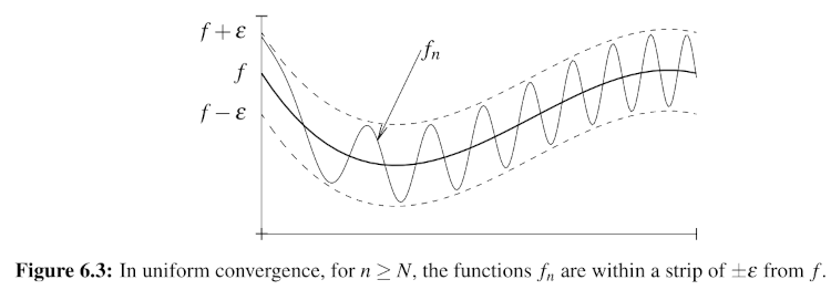
An illustration how $f_n$ is bounded to the $\epsilon$ window and as $\epsilon$ gets smaller, the $f_n$ gets squeezed but remains in the window. i.e. Eventually as you go further down the sequence (a larger $N$), you will eventually find a function flat enough to squeeze into the window. Extracted from MIT OCW Real Analysis Notes

Now we have seen what it means for a function to converge pointwise and uniformly, let us now revisit the purpose of introducing a strongegr notion of convergence (uniform convergence):

$f_n$ is continuous $\forall n$ and $f_n \to f$ pointwise $\bcancel{\implies} f$ is continuous

But

$f_n$ is continuous $\forall n$ and $f_\to f$ uniformly $\implies f $ is continuous

Theorem (Uniform Convergence Preserving Continuity): let $(f_n)$ be a sequence of functions on $S$ such that $f_n \to f$ converges uniformly. If each $f_n$ is continuous, so is $f$

If we take the contrapositive of this theorem above, we obtain another tool to disprove uniform convergence:

Disproving Uniform Convergence via Continuity: If $f_n \to f$ pointwise and each $f_n$ is continuous but $f(x)$ is not continuous, then this convergence is not uniform

Before proceeding to the consequences of uniform convergence and the preservation of continuity, let’s revisit our favorite function in this chapter: $f_n(x) = x^n$ and recall that $f_n \to f$ pointwise on $[0,1]$ where,

\[f(x) = \begin{cases} 0 & x\in[0,1) \nonumber\\ 1 & x = 1 \end{cases}\]

This does not uniformly converge to $f$ as it was discontinuous at $x = 1$. But what about for $x\in[0,1)$?

For $f_n = x^n$ on $[0,1), \lim\limits_{n\to\infty} f_n(x) = 0 \forall x$

The constant function $0$ is continuous $\forall x$ but is it uniformly convergent on $[0,1)$? NO, we showed previously that it did not

What about from a fixed positive number $b \lt 1$. We will make the claim that on $[0,b], f_n \to 0$ uniformly:

Rough Work: Let $\epsilon \gt 0$. We want $N$ such that $n \gt N$:

\[\begin{align*} |x^n - 0| \lt \epsilon \forall x\in [0,b] \\ |x^n| = x^n \leq b^n \underset{\text{want}}{\lt} \epsilon \end{align*}\]

Note: $b^n \lt \epsilon$ is only possible because $b \lt 1$ thus $b^n \lt 1$ (i.e. for $b\lt 1 \implies b^{N+1} \lt b^{N}$)

Thus we have,

\[\begin{align*} b^n \lt \epsilon &\iff n\ln b \lt \ln \epsilon \\ &\iff n \gt \frac{\ln\epsilon}{\ln b}, \quad \text{inequality flipped because if $b\lt 1$ then $\ln b \lt 0$} \end{align*}\]

Thus choose $N = \frac{\ln\epsilon}{\ln b}$

In conclusion, for the examples, we have seen for $f_n(x) = x^n$,

\(f(x) = \begin{cases} 0 & 0\leq x \lt 1 \\ 1 & x = 1 \end{cases}\)

• on $[0,1], f_n \to f$ pointwise but not uniformly
• on $[0,1), f_n \to 0$ pointwise but not uniformly
• on $[0,b]$ for $b \lt 1, f_n \to 0$ uniformly

I recall being a bit surprised by this result how fixing a point allows $f_n$ converge uniformly to $f$. But now that I think of it, if we were to start plugging in numbers as $x \to 1$, we’ll notice the following:

• $x = 0.5: 0.5^n \to 0$ fast ($N_1 > N$)
• $x = 0.9: 0.9^n \to 0$ slowly (i.e. $N_2 » N_1 > N$)
• $x = 0.99: 0.99^n \to 0$ even slower (i.e. $N_3 »> N_2 » N_1 > N$)
• $x \to 1: x^n \to 0$ extremely and arbitrarily slowly (i.e. $N_4 »»»»»»» N_3 »> N_2 » N_1 > N$)

Thus as $x\to 1$, we observe the growth to converge $f_n(x)$ to 0 get slower and slower

We can now say the following:

Theorem: let $(t_n)$ be a sequence of continuous function on $[a,b]$ which converges uniformly to $f$.

Then $\lim\limits_{n\to\infty} \int_a^b f_n(x)dx = \int_a^b \lim\limits_{n\to\infty} f_n(x)dx = \int_a^b f(x)dx$

Previously, we saw that $f_n = x^n$ does not converge uniformly from [0,1) as the terms converges to $f$ so slowly. In MATH1052, we introduced cauchy sequences, a sequence that converges and exhibits a behavior whereby after some $N$, the distance of any two functions in the sequence are arbitrarily so close that convergence is guaranteed.

Cauchy Sequences: a sequence $(s_n)$ is cauchy if $\forall \epsilon \gt 0, \exists N $ such that $m,n \gt N \implies |a_n-a_m| \lt \epsilon$

$(s_n)$ is cauchy $\iff (s_n)$ is convergent

We want a similar result for functions because if you recalled, this entire section is dedicated to power series which are infinite series of functions (even though it may not seem like it with our discussion in sequences and convergence).

Uniformly Cauchy: a sequence $(f_n)$ of functions on $S\subseteq \mathbb{R}$ is called UNIFORMLY CAUCHY if $\forall \epsilon \gt 0, \exists N$ such that $m,n \gt N \implies |f_n(x) - f_m(x)| \lt \epsilon \quad\forall x\in S$

To tie this together with uniform convergent, we have the following result:

Lemma: if $f_n \to f$ uniformly then it is uniformly cauchy

and

Theorem: Let $(f_n)$ be a uniformly cauchy sequence of functions on $S\subseteq \mathbb{R}$ then $\exists$ a function $f$ on $S$ such that $f_n\to f$ uniformly

Thus far, we have talked about functions in a sequence but never tied it with power series. Let us now be equipped with what it means for a series of functions to a power series:

$\sum\limits_{k = 0}^\infty g_k(x)$ is a power series of functions if $g_k(x) = a_kx^k$

For instance, the following function is a series of function but is not a power series of functions: $\sum\limits_{k=0}^\infty \frac{x^k}{1+x^k}$ because it is not in the right form.

Uniform Convergence of Function Power Series: let $\sum\limits_{k=0}^\infty g_k(x)$ be a series of functions on $S$ such that each $g_k$ is continuous. If $\sum\limits_{k=0}^\infty g_k(x)$ is uniformly convergent to $g(x)$, then $g$ is continuous

This result should not be of any surprise as we previously saw that

• sums of continuous functions are continuous
• uniform convergence preserves continuity among convergent sequences of functions

Let us now introduce another equivalence relation to uniformly cauchy in respect to function power series:

Uniform Cauchy Definition for $\sum\limits_{k=0}^\infty g_k(x)$: $\sum\limits_{k=0}^\infty g_k(x)$ is uniformly cauchy on $S$

$\iff \forall \epsilon \gt 0, \exists N $ such that $m,n \gt N \implies |\sum\limits_{k=0}^n g_k(x) - \sum\limits_{k=0}^m g_k(x)|\lt \epsilon$

$\iff \forall \epsilon \gt 0, \exists N $ such that $n\geq m \gt N \implies |\sum\limits_{k=m}^n g_k(x)| \lt \epsilon$

Now that we have seen what it means for a power series to uniformly converge, we can now introduce a nice test to determine whether it converges uniformly:

Weierstrass M-Test: let $(M_K)$ be a sequence of non-negative numbers with $\sum\limits_{k=0}^\infty M_k \lt \infty$. If $|g_k(x)| \leq M_k \forall x\in S$, then $\sum\limits_{k=0}^\infty g_k(x)$ converges uniformly on $S$

Let us see an example of how to utilise this test to determine whether an infinite function power series converges ot a continuous function:

Example: Show that $\sum\limits_{k=0}^\infty \frac{1}{n^2}\sin(nx)$ converges to a continuous function on $\mathbb{R}$

First note that: $|\frac{1}{n^2}\sin(nx)| = \frac{1}{n^2}|\sin(nx)|\leq \frac{1}{n^2}$

Let $M_n = \frac{1}{n^2}$. Then $\sum\limits_{k=0}^\infty M_n = \sum\limits_{k=0}^\infty \frac{1}{n^2} \lt \infty$ by P-series

So by M-test, $\sum\limits_{k=0}^\infty \frac{1}{n^2}\sin(nx)$ converges uniformly on $\mathbb{R}$ Since $g_n(x) = \frac{1}{n^2}\sin(nx)$ is continuous on $\mathbb{R} \forall n$ and converges uniformly, the limit must be continuous.

Recall: if $\sum\limits_{k=0}^\infty a_k$ is a series of numbers then $\sum\limits_{k=0}^\infty a_k$ converges $\implies \lim\limits_{n\to\infty} a_n = 0$

Though the opposite direction does not hold (think of $\sum \frac{1}{n}$ diverges by P-series but the limit is 0. We have an analogous version of this fact for series of functions:

if $\sum\limits_{k=0}^\infty g_k(x)$ converges uniformly on $S$ then $\lim\limits_{n\to\infty} \sup\{|g_n(x)| : x\in S\} = 0$

One consequence of this lemma above is that we can use the contrapositive to conclude whether a function power series does not converge uniformly, which is probably a much more useful fact:

if one can show $\lim\limits_{n\to\infty} \sup\{|g_n(x)| : x\in S\} \neq 0$, then one can conclude that $\sum g_k(x)$ does not converge uniformly on $S$

Example: Consider the power series $\sum \frac{x^n}{3^n}$

Before utilising our new tool to determine whether this power series converges uniformly, let’s establish the convergence interval:

Note that the radius of convergence is 3: $R = \lim\limits_{n\to\infty}\left|\frac{a_n}{a_{n+1}}\right| = \left|\frac{\frac{1}{3^n}}{\frac{1}{3^{n+1}}}\right| = 3$

At $x = 3: \sum 1 = \infty$ and at $x = -3: \sum(-1)^n$ diverges. Thus our interval of convergence is: $I = (-3,3)$

Using the new tool, we have $\sup\{|\frac{x^n}{3^n}| : x\in (-3,3)\} = 1 \forall n$ so $\lim_{x\to\infty} \sup\{|\frac{x^n}{3^n}| : x\in (-3,3)\} = 1 \neq 0$

So by the lemma, we know $\sum \frac{x^n}{3^n}$ does not converge uniformly on $(-3,3)$

But what if we restricted the interval to a concrete number similar to how we found $f_n(x) = x^n$ converges uniformly if we restricted $S$ from $[0,1)$ to $[0, b]$. It turns out if we restrict the endpoints of our interval of convergence to be smaller and concrete, our once non-uniformly convergent sequence/power series does converge.

Theorem: let $\sum a_n x^n$ be a power series with a radius of convergence $R \gt 0$. If $0 \lt b \lt R$, then the power series converges uniformly on $[-b,b]$ and converges to a continuous function on $(-R,R)$

Let’s revisit the previous example and restrict the interval to $b \lt R = 3$. For this exercise, we will avoid invoking the theorem above and show you the lengthy process to obtain the same result:

Let $b\in(0,3)$ so if $x = b\implies \sum \frac{b^n}{3^n} = \sum\left(\frac{b}{3}\right)^n$ converges by gemoetric series (as $0 \lt b \lt 3$)

1. To show $\sum \frac{x^n}{3^n}$ converges uniformly on $[-b,b]$, we can utilise the Weierstrass M-test: $\forall x\in [-b,b], \left|\frac{x^n}{3^n} \right | \leq \left|\frac{b^n}{3^n}\right| = \left(\frac{b}{3}\right)^n = M_n$. Since $\sum M_n$ converges, by the Weierstrass M-test, $\sum\frac{x^n}{3^n}$ converges uniformly on $[-b,b]$.

2. Now all that is left is to show $\sum \frac{x^n}{3^n}$ converges to a continuous function on $[-b,b]$:

   Note that $\frac{x^n}{3^n}$ is continuous on $\forall n$. Thus, $\sum\frac{x^n}{3^n}$ is continuous on $[-b,b] \forall b\in[0,3)$. As $b$ is arbitrary, $\sum \frac{x^n}{3^n}$ converges to a continuous function on $(-3, 3)$.

This is definitely much longer than simply invoking the theorem which gives us both uniformly convergence and convergence to a continuous function for free: Since $R = 3 \gt 0$ and $b \in (0,R)$, by the theorem above, we have $\sum \frac{x^n}{3^n}$ converges uniformly on $[-b,b]$ and converges to a continuous function on $(-3,3)$.

Recall that one of the motivations of utilising power series is to represent transcendental functions such as $e^x$ as an infinite series of polynomials. What would be desirable is if we could differentiate and integrate power series term by term. For instance, it would be nice if we could do the following

\[\begin{align*} \left(\sum\limits_{n=0}^\infty a_nx^n\right)' &= (a_0 + a_1x + a_2x^2+\cdots)' \overset{?}{=} a_1 + 2a_2x+3a_3x^2+\cdots \overset{?}{=} \sum\limits_{n=1}^\infty na_nx^{n-1} \\ \int \sum\limits_{n=0}^\infty a_nx^ndx &\overset{?}{=} \sum\limits_{n=0}^\infty \frac{a_nx^{n+1}}{n+1} \end{align*}\]

But for these properties to work, we must ensure that the radius of convergence remains the same in these new forms:

Lemma: If $\sum\limits_{n=0}^\infty a_n x^n$ has a radius of convergence $R$, then so does $\sum\limits_{n=1}^\infty na_nx^{n-1}$ and $\sum\limits_{n=0}^\infty \frac{a_n}{n+1}x^{n+1}$

As the radius of convergence remains the same even after taking the form of what seems like to be its differentiatiable and integrable equivalences, let us now introduce the theorem that ties this together to permit us to integrate and differentiate the series term by term:

Theorem: Suppose $f(x) = \sum_{n=0}^\infty a_nx^n$ has a radius of convergence $R \gt 0$. Then, $\int_0^x f(t)dt = \sum\limits_{n=0}^\infty \frac{a_n}{n+1}x^{n+1}$ for $|x| \lt R$

Theorem: Let $f(x) = \sum_{n=1}^\infty a_nx^n$ have radius of convergence $R \gt 0$. Then $f$ is differentiable on $(-R,R)$ and

$f’(x) = \sum_\limits{n=1}^\infty na_nx^{n-1}$ for $|x| \lt R$

Note: Notice that the index changes from 0 to 1 in the differentiable form. The index does not change for the integral

Thus far. the previous theorem only discusses differentiablity at the open intervals $(-R, R)$ but what about at its endpoint? That is what the next theorem, Abel’s Theorem, attempts to tackle. We know from last year that differentiability implies continuity (i.e. to be differentiable at $x = a$, then by definition, it must also be continuous at $a$)

Abel’s Theorem: let $f(x) = \sum a_nx^n$ have a radius of convergence $R \gt 0$, $R \lt \infty$. If $\sum a_nx^n$ converges at $x = R$, then it is continuous there. The same is true at $x = -R$.

As a consequence, we have that every power series converge to a continuous function on its entire interval of convergence including at its endpoint provided it is defined and does indeed converge there.

Every power series converges to a continuous function on its entire interval of convergence (including its endpoints if defined and converges there)

i.e. $\sum \frac{x^n}{n^2}$ has an interval of convergence (I.O.C) on $[-1,1]$ and thus is continuous on $[-1,1]$

---

Taylor Series

Recall that one of the motivations of power series is to represent transcendental functions as an infinite series of polynomials. This is the math that allows calculators be able to compute $e^x$ for instance within an acceptable error or to allow oneself to integrate a complicated expression into simple series of polynomials. However, how does one translate a function such as $e^x$ or $\sin(x)$ into a series of polynomials? That is what will be explored in this section, working with taylor series which gives us a methodical way to transform a function into a power series.

Taylor Series: let $f$ be defined on an open interval containing $x_o$. Suppose that all order of derivatives of $f$ exist at $x_o$. Then the series

$\sum\limits_{n=0}^\infty \frac{f^{(n)}(x_o)}{n!}\left(x-x_o\right)^n$ is called the taylor series for $f$ about $x_o$

For $n\geq 1$, the remainder $R_n(x)$ is defined by:

$R_n(x) = f(x) - \sum\limits_{k=0}^{n-1}\frac{f^{(k)}(c)}{k!}(x-c)^k$

When we approximate a function $f(x)$ using a finite Taylor polynomial of degree $n$ which we call $P_n(x)$, the approximation is rarely perfect. This difference must be taken into account and thus the remainder

\[\begin{align*} R_n(x) &= f(x) - \sum\limits_{k=0}^{n-1} \frac{f^{(k)}(c)}{k!}(x-c)^k \\ f(x) &= \sum\limits_{k=0}^{n-1} \frac{f^{(k)}(c)}{k!}(x-c)^k + R_n(x) \\ f(x) &= P_n(x) + R_n(x) \end{align*}\]

On a note about the remainder, we also have this result:

$f(x) = \sum\limits_{k=0}^\infty \frac{f^{(n)}(x_o)}{k!}(x-x_o)^n \iff \lim\limits_{n\to\infty}R_n(x) = 0$

Suppose we have a power series in the form $f(x) = \sum a_n(x-x_o)^n$. We have never discussed how to determine what $a_n$ is. In our definition of taylor series, all order of derivatives of $f$ exists at $x_o$. This,

\[\begin{align*} f(x) &= a_o + a_1(x-x_o) + a_2(x-x_o)^2 + a_3(x-x_o)^3 + \cdots \\ f'(x) &= a_1 + 2a_2(x-x_o) + 3a_3(x-x_o)^2 + \cdots \\ f''(x) &= 2a_2 + (3)(2)a_3(x-x_o) + 4(3)a_4(x-x_o)^2 + \cdots \\ f'''(x) &= 3(2)a_3 + 4(3)(2)a_4(x-x_o) + 5(4)(3)a_5(x-x_o)^2 + \cdots \end{align*}\]

Let $x = x_o$, then:

\[\begin{align*} f(x_o) &= a_o &= 0!a_o \\ f'(x_o) &= a_1 &= 1! a_1 \\ f''(x_o) &= 2a_2 &= 2!a_2 \\ f'''(x_o) &= 3(2)a_3 &= 3! a_3 \end{align*}\]

Then by induction, we have:

\[\begin{align*} f^{(n)} = n!a_n\\ \boxed{a_n = \frac{f^{(n)}(x_o)}{n!}} \end{align*}\]

Taylor Coefficient: $a_n = \frac{f^{(n)}(x_o)}{n!}$

Let us now go through an example to determine the taylor series of $\sin(x)$ centered at 0 (Note: This is also called a Maclaurin Series, a Taylor series centered at 0).

First let’s observe the orders of the derivatives of $\sin(x)$:

\[\begin{align*} f(x) &= \sin(x) & f(0) &= 0 \\ f'(x) &= \cos(x) & f'(0) &= 1 \\ f''(x) &= -\sin(x) & f''(0) &= 0 \\ f^{(3)}(x) &= -\cos(x) & f^{(3)}(0) &= -1 \\ f^{(4)}(x) &= \sin(x) & f^{(4)}(0) &= 0 \\ \cdots \end{align*}\]

So we have: \(f^{(n)}(0) = \begin{cases} 0 & \text{if n is even} \\ 1 & \text{if n = 4k+1} \\ -1 & \text{if n = 4k+3} \end{cases}\)

and $a_n = \frac{f^{(n)}(0)}{n!}$ so the taylor series of $\sin(x)$ around 0 is

\[\begin{align*} \sum\limits_{k=0}^\infty \frac{f^{(k)}(0)}{k!}x^k &= x - \frac{x^3}{3!} + \frac{x^5}{5!} - \frac{x^7}{7!} + \cdots \\ &= \sum\limits_{n=0}^\infty \frac{(-1)^nx^{2n+1}}{(2n+1)!} \end{align*}\]

Let’s now explore the one applications of taylor series I hinted at in the beginning to better understand the power of formulating a function as a taylor series:

For Approximations:

How many terms do we need to approximate $\sqrt{e} = e^\frac{1}{2} = \sum\limits_{n=0}^\infty \frac{\left(\frac{1}{2}\right)^n}{n!}$ with an error less than $0.0001$?

Recall that $e^x = \sum\limits_{k=0}^\infty \frac{x^k}{k!} = \sum\limits_{k=0}^{n-1} \frac{x^k}{k!} + R(x)$

where $R_n(x) = \frac{f^{(n)}(y)}{n!}x^n = \frac{e^y}{n!}x^n$ for some $y\in(0,x)$

Since we are evaluate for $e^\frac{1}{2} = e^x \implies x = \frac{1}{2}$:

\[R_n\left(\frac{1}{2}\right) = \frac{e^y}{n!}\left(\frac{1}{2}\right)^n = \frac{e^y}{2^nn!}, y\in\left(0,\frac{1}{2}\right) \nonumber\]

So a crude estimate would be that $e \lt 3$ (recall $e = 2.71828\cdots$)

We can bound $e^\frac{1}{2}$:

\[e^y \lt e^\frac{1}{2} \lt 3^\frac{1}{2} \lt 2 \nonumber\]

So we can bound the remainder:

\[\begin{align*}|R_n\left(\frac{1}{2}\right)| \lt \frac{2}{2^nn!} = \frac{1}{n!2^{n-1}} &\overset{\text{want}}{\lt} 0.0001\\ \iff 10000 &\lt n!2^{n-1} \end{align*}\]

If we were to iterate, the first time this condition holds true is when $n = 6$ and thus the error is less than $\frac{1}{6!2^5} \approx 0.000043$

While this does not give as the true error, it is nonethless cool that we can bound the error using what we know about Taylor series.

There are plenty more applications of taylor series such as solving tough integrals, solving the Basel problem, and solving differential equations. But that is all for this topic and my commentary on the course materials.

---

Resources

• MATH2052 Notes from Charles Starling
• Elementary Analysis: The Theory of Calculus by Kenneth A. Ross
• MIT OCW Real Analysis Notes

Note: I refer to this page as a commentary to the course or an accompanying to the course, these are not class notes. I the author of this page will omit many details and only present the materials and proofs to things I find personally noteworthy and the proofs presented may differ from those listed in the textbook or from the course notes itself.

---

Note: The reviews are bias and reflects my perception of the course. In addition, the information varies depending on the professor and will likely be outdated.

---

For More Bias Course Reviews:

• MATH2052 - A Commentary on Calculus and Introductory Analysis 2
• MATH1052 - A Commentary on Calculus and Introductory Analysis 1
• MATH3001 - Real Analysis 1
• MATH1800 - Introduction to Mathematical Reasoning
• MATH2000 - Multivariable Calculus and Fundamentals of Analysis [Fall+Winter]
• PHYS1004 - A Review on Introductory Electromagnetism and Wave Motion
• MATH2107 - Linear Algebra II
• MATH2052 - Calculus and Introductory Analysis II
• PHYS1001 - A Review on Foundations of Physics 1
• MATH1152 - Introductory Algebra 1
• MATH1052 - Calculus and Introductory Analysis 1
• Bias UTM CS Course Review